scRNAseq_combined_01_preprocessing
retogerber
2022-12-19
Last updated: 2022-12-19
Checks: 6 1
Knit directory: synovialscrnaseq/
This reproducible R Markdown analysis was created with workflowr (version 1.6.2). The Checks tab describes the reproducibility checks that were applied when the results were created. The Past versions tab lists the development history.
The R Markdown is untracked by Git. To know which version of the R Markdown file created these results, you’ll want to first commit it to the Git repo. If you’re still working on the analysis, you can ignore this warning. When you’re finished, you can run wflow_publish to commit the R Markdown file and build the HTML.
Great job! The global environment was empty. Objects defined in the global environment can affect the analysis in your R Markdown file in unknown ways. For reproduciblity it’s best to always run the code in an empty environment.
The command set.seed(20210105) was run prior to running the code in the R Markdown file. Setting a seed ensures that any results that rely on randomness, e.g. subsampling or permutations, are reproducible.
Great job! Recording the operating system, R version, and package versions is critical for reproducibility.
Nice! There were no cached chunks for this analysis, so you can be confident that you successfully produced the results during this run.
Great job! Using relative paths to the files within your workflowr project makes it easier to run your code on other machines.
Great! You are using Git for version control. Tracking code development and connecting the code version to the results is critical for reproducibility.
The results in this page were generated with repository version 816d5c9. See the Past versions tab to see a history of the changes made to the R Markdown and HTML files.
Note that you need to be careful to ensure that all relevant files for the analysis have been committed to Git prior to generating the results (you can use wflow_publish or wflow_git_commit). workflowr only checks the R Markdown file, but you know if there are other scripts or data files that it depends on. Below is the status of the Git repository when the results were generated:
Ignored files:
    Ignored:    '/
    Ignored:    .Rhistory
    Ignored:    .Rproj.user/
    Ignored:    .empty/
    Ignored:    analysis/.Rhistory
    Ignored:    analysis/iSEE_interactive_document.html
    Ignored:    code/test_files/
    Ignored:    data/Culemann/
    Ignored:    data/E-MTAB-8322/
    Ignored:    data/Synovial scRNA-seq samples - Sheet1.csv
    Ignored:    data/Zhang_top20_singlecell_cluster_markers_fromGithub.csv
    Ignored:    data/findMarkers_results.rds
    Ignored:    data/findMarkers_results_v2.rds
    Ignored:    data/info/
    Ignored:    data/syn_sce_tidy_filtered.rds
    Ignored:    data/syn_sce_tidy_hvg.rds
    Ignored:    data/syn_sce_tidy_hvg_cms.rds
    Ignored:    docs/
    Ignored:    output/Figures_Paper/
    Ignored:    output/Sample_summaries_RA_comparisons.rds
    Ignored:    output/Sample_summaries_direct_dissociation.rds
    Ignored:    output/Sample_summaries_exvivo_treatment.rds
    Ignored:    output/Suppl_Figure_4d.rds
    Ignored:    output/barcodes.txt
    Ignored:    output/combined_v7_sce.rds
    Ignored:    output/combined_v7_sce_filtered.rds
    Ignored:    output/combined_v7_sce_hvg.rds
    Ignored:    output/combined_v7_upsetplot_genelists.rds
    Ignored:    output/count_matrix_unfiltered.mtx
    Ignored:    output/emptyDrops_result_v4.rds
    Ignored:    output/emptyDrops_result_v4_tmp.rds
    Ignored:    output/emptyDrops_result_v4tmptmp.rds
    Ignored:    output/entropies_fstat_v5_ec.rds
    Ignored:    output/entropies_fstat_v5_main.rds
    Ignored:    output/entropies_fstat_v5_mp.rds
    Ignored:    output/entropies_fstat_v5_sf.rds
    Ignored:    output/entropies_fstat_v5_tc.rds
    Ignored:    output/findMarkers_results_v5_ec.rds
    Ignored:    output/findMarkers_results_v5_main.rds
    Ignored:    output/findMarkers_results_v5_mp.rds
    Ignored:    output/findMarkers_results_v5_sf.rds
    Ignored:    output/findMarkers_results_v5_tc.rds
    Ignored:    output/findMarkers_results_v6.rds
    Ignored:    output/findMarkers_results_v6_ec.rds
    Ignored:    output/findMarkers_results_v6_main.rds
    Ignored:    output/findMarkers_results_v6_mp.rds
    Ignored:    output/findMarkers_results_v6_sf.rds
    Ignored:    output/findMarkers_results_v6_tc.rds
    Ignored:    output/findMarkers_results_v7_ec.rds
    Ignored:    output/findMarkers_results_v7_main.rds
    Ignored:    output/findMarkers_results_v7_mp.rds
    Ignored:    output/findMarkers_results_v7_sf.rds
    Ignored:    output/findMarkers_results_v7_tc.rds
    Ignored:    output/genes.txt
    Ignored:    output/goana_results_v6_ec.rds
    Ignored:    output/goana_results_v6_mp.rds
    Ignored:    output/preprocessing_number_of_cells.rds
    Ignored:    output/syn_v4_sce_emptyDrops_invivo.rds
    Ignored:    output/syn_v4_swappedDrops_24300_after.rds
    Ignored:    output/syn_v4_swappedDrops_24300_before.rds
    Ignored:    output/syn_v4_swappedDrops_24793_after.rds
    Ignored:    output/syn_v4_swappedDrops_24793_before.rds
    Ignored:    output/syn_v5_annot_df_manual.rds
    Ignored:    output/syn_v5_cluster_cellid_match_invivo.rds
    Ignored:    output/syn_v5_clustering_lookup_invivo.rds
    Ignored:    output/syn_v5_clustering_lookup_multiple_invivo.rds
    Ignored:    output/syn_v5_res_da_Accute_inflammation_invivo.rds
    Ignored:    output/syn_v5_res_da_Diagnosis_invivo.rds
    Ignored:    output/syn_v5_res_da_Diagnosis_main_invivo.rds
    Ignored:    output/syn_v5_res_da_Lymphoid_folicles_invivo.rds
    Ignored:    output/syn_v5_res_da_Pathotype_invivo.rds
    Ignored:    output/syn_v5_res_da_Therapy_invivo.rds
    Ignored:    output/syn_v5_res_da_Vascularisation_bin_invivo.rds
    Ignored:    output/syn_v5_res_ds_Accute_inflammation_invivo.rds
    Ignored:    output/syn_v5_res_ds_Diagnosis_invivo.rds
    Ignored:    output/syn_v5_res_ds_Diagnosis_main_invivo.rds
    Ignored:    output/syn_v5_res_ds_Lymphoid_folicles_invivo.rds
    Ignored:    output/syn_v5_res_ds_Pathotype_invivo.rds
    Ignored:    output/syn_v5_res_ds_Therapy_invivo.rds
    Ignored:    output/syn_v5_res_ds_Vascularisation_bin_invivo.rds
    Ignored:    output/syn_v5_sce.rds
    Ignored:    output/syn_v5_sce_ec_invivo.rds
    Ignored:    output/syn_v5_sce_filtered_invivo.rds
    Ignored:    output/syn_v5_sce_hvg_cms_doublet_annot_manual_invivo.rds
    Ignored:    output/syn_v5_sce_hvg_cms_doublet_cmstest_invivo.rds
    Ignored:    output/syn_v5_sce_hvg_cms_doublet_invivo.rds
    Ignored:    output/syn_v5_sce_hvg_cms_doublet_subcluster_invivo.rds
    Ignored:    output/syn_v5_sce_hvg_invivo.rds
    Ignored:    output/syn_v5_sce_mp_invivo.rds
    Ignored:    output/syn_v5_sce_sf_invivo.rds
    Ignored:    output/syn_v5_sce_tc_invivo.rds
    Ignored:    output/syn_v5_vst_out_invivo.rds
    Ignored:    output/syn_v6_cluster_cellid_match_invivo.rds
    Ignored:    output/syn_v6_clustering_lookup_invivo.rds
    Ignored:    output/syn_v6_clustering_lookup_multiple_invivo.rds
    Ignored:    output/syn_v6_sce.rds
    Ignored:    output/syn_v6_sce_Figure8.rds
    Ignored:    output/syn_v6_sce_Figure8_dic_ls.rds
    Ignored:    output/syn_v6_sce_ec_invivo.rds
    Ignored:    output/syn_v6_sce_filtered_invivo.rds
    Ignored:    output/syn_v6_sce_hdf5/
    Ignored:    output/syn_v6_sce_hvg_cms_doublet_invivo.rds
    Ignored:    output/syn_v6_sce_hvg_cms_doublet_subcluster_invivo.rds
    Ignored:    output/syn_v6_sce_hvg_invivo.rds
    Ignored:    output/syn_v6_sce_hvg_marker_genes.rds
    Ignored:    output/syn_v6_sce_mp_invivo.rds
    Ignored:    output/syn_v6_sce_sf_invivo.rds
    Ignored:    output/syn_v6_sce_tc_invivo.rds
    Ignored:    output/syn_v6_sfig1.rds
    Ignored:    output/syn_v6_vst_out_invivo.rds
    Ignored:    output/syn_v7_cluster_cellid_match_invivo.rds
    Ignored:    output/syn_v7_clustering_lookup_invivo.rds
    Ignored:    output/syn_v7_clustering_lookup_multiple_invivo.rds
    Ignored:    output/syn_v7_sce.rds
    Ignored:    output/syn_v7_sce_ec_invivo.rds
    Ignored:    output/syn_v7_sce_filtered_invivo.rds
    Ignored:    output/syn_v7_sce_hdf5/
    Ignored:    output/syn_v7_sce_hvg_cms_doublet_invivo.rds
    Ignored:    output/syn_v7_sce_hvg_cms_doublet_subcluster_invivo.rds
    Ignored:    output/syn_v7_sce_hvg_invivo.rds
    Ignored:    output/syn_v7_sce_mp_invivo.rds
    Ignored:    output/syn_v7_sce_sf_invivo.rds
    Ignored:    output/syn_v7_sce_tc_invivo.rds
    Ignored:    output/syn_v7_sfig1.rds
    Ignored:    output/syn_v7_vst_out_invivo.rds

Untracked files:
    Untracked:  analysis/scRNAseq_combined_01_preprocessing.Rmd
    Untracked:  analysis/scRNAseq_combined_02_HVG_Dimred.Rmd
    Untracked:  analysis/scRNAseq_combined_03_Batch.Rmd
    Untracked:  analysis/scRNAseq_combined_04_labels.Rmd
    Untracked:  analysis/scRNAseq_complete_01_preprocessing_comparison.Rmd
    Untracked:  analysis/scRNAseq_complete_04_Annotation_v7.Rmd
    Untracked:  analysis/test.Rmd
    Untracked:  code/rebuild_ezRun.R
    Untracked:  nonhosted_public/
    Untracked:  singRstudio.sh.bak

Unstaged changes:
    Modified:   analysis/scRNAseq_complete_01_preprocessing.Rmd
    Modified:   analysis/scRNAseq_complete_02_HVG_Dimred.Rmd
    Modified:   analysis/scRNAseq_complete_03-2_Subcelltypes_processing.Rmd
    Modified:   analysis/scRNAseq_complete_03-3_Subcelltypes_clustering.Rmd
    Modified:   analysis/scRNAseq_complete_03-4_Subcelltypes_clustering_walktrap.Rmd
    Modified:   analysis/scRNAseq_complete_03_Batch_Clustering_Doublets.Rmd
    Modified:   analysis/scRNAseq_complete_04-2_celltype_markers.Rmd
    Modified:   analysis/scRNAseq_complete_04-2_celltype_markers_subcelltypes.Rmd
    Modified:   analysis/scRNAseq_complete_Figures.Rmd
    Modified:   analysis/write_tsv.Rmd
    Modified:   code/create_hdf5.R

Staged changes:
    Modified:   analysis/scRNAseq_complete_00_ambient_RNA.Rmd
Note that any generated files, e.g. HTML, png, CSS, etc., are not included in this status report because it is ok for generated content to have uncommitted changes.
There are no past versions. Publish this analysis with wflow_publish() to start tracking its development.
Set up
suppressPackageStartupMessages({
  library(dplyr)
  library(purrr)
  library(scater)
  library(scran)
  library(scuttle)
  library(tidySingleCellExperiment)
  library(BiocParallel)
})

n_workers <- 10
RhpcBLASctl::blas_set_num_threads(n_workers)
bpparam <- BiocParallel::MulticoreParam(workers=n_workers, RNGseed = 123)

analysis_version <- 7
here::here()
[1] "/home/retger/Synovial/synovialscrnaseq"raw_data_dir <- here::here("..","data_server")
raw_data_dir_wei <- here::here("..","data_wei")
raw_data_dir_stephenson <- here::here("..","data_stephenson")
source(here::here("code","utilities_plots.R"))
set.seed(100)Read Raw counts
Wei
dirs_wei <- c("RA1","RA2","RA3","RA4","RA5","RA6")
# prepare
samples_wei <- here::here(raw_data_dir_wei,dirs_wei,"outs","filtered_feature_bc_matrix")
names(samples_wei) <- dirs_wei

sce_wei_ls <- lapply(
                                 seq_along(samples_wei),
                                 function(i){
  sce_tmp <- DropletUtils::read10xCounts(samples=samples_wei[i], sample.names=paste0("W_",names(samples_wei[i])), type="sparse")
  colnames(sce_tmp) <- paste0(sce_tmp$Sample, ".", sce_tmp$Barcode)
  rownames(sce_tmp) <- paste0(rowData(sce_tmp)$ID, ".", rowData(sce_tmp)$Symbol)
  sce_tmp$Diagnosis <- "Rheumatoid_Arthritis"
  sce_tmp$Protocol <- "wei"
  sce_tmp$Joint <- NA
  sce_tmp$Sample_prep <- "frozen"
  sce_tmp
})
Stephenson
countmat_stephenson <- read.csv(here::here(raw_data_dir_stephenson, "RA_5Knees_Expression_Matrix.tsv"), header = TRUE, sep = ",")
countmat_mat_stephenson <- as.matrix(countmat_stephenson[,-1])
rownames(countmat_mat_stephenson) <- countmat_stephenson[,1]
Sample <- colnames(countmat_mat_stephenson) %>% stringr::str_extract("RA[:digit:]+")
Barcode <- colnames(countmat_mat_stephenson) %>% stringr::str_extract("(?<=RA[:digit:]{1}_)[:alnum:]+")
Symbol <- rownames(countmat_mat_stephenson)

sce_stephenson <- SingleCellExperiment(assays=SimpleList(counts=countmat_mat_stephenson),
                     colData=DataFrame(row.names = colnames(countmat_mat_stephenson),
                                       Sample = paste0("S_",Sample),
                                       Barcode = Barcode,
                                       Diagnosis = "Rheumatoid_Arthritis",
                                       Protocol = "stephenson",
                                       Joint = NA,
                                       Sample_prep = "fresh"),
                     rowData=DataFrame(Symbol=Symbol))
combine
syn_sce <- purrr::reduce(sce_wei_ls, cbind)

# add Stephenson data
tmpind <- rowData(sce_stephenson)$Symbol %in% rowData(syn_sce)$Symbol
tmpind2 <- rowData(syn_sce)$Symbol %in% rowData(sce_stephenson)$Symbol
sce_stephenson <- sce_stephenson[tmpind,]
syn_sce <- syn_sce[tmpind2,]
genematch <- match(rowData(syn_sce)$Symbol,rowData(sce_stephenson)$Symbol)
genematch <- genematch[!is.na(genematch)]
all(rowData(sce_stephenson)$Symbol[genematch] == rowData(syn_sce)$Symbol)

syn_sce <- cbind(syn_sce, sce_stephenson[genematch,])
colnames(syn_sce) <- make.unique(colnames(syn_sce),".")


# number of cells
table(colData(syn_sce)$Sample)

# filter genes and cells, genes have to be expressed in at least 1% of cells, and
# cells need at least 250 counts
one_perc_cells <- ceiling(dim(syn_sce)[2]/100/length(unique(syn_sce$Sample)))
print(one_perc_cells)
dim(syn_sce)
syn_sce  <- syn_sce[rowSums(counts(syn_sce) > 0) > one_perc_cells,
                              colSums(counts(syn_sce) > 0) > 250]
dim(syn_sce)
syn_sce  <- syn_sce[rowSums(counts(syn_sce) > 0) > one_perc_cells,
                              colSums(counts(syn_sce) > 0) > 250]
dim(syn_sce)
Doublet detection
Run scDblFinder.
bpstart(bpparam)
syn_sce <- scDblFinder::scDblFinder(syn_sce,
                                                 samples=syn_sce$Sample,
                                                 BPPARAM = bpparam)
bpstop(bpparam)
table(syn_sce$scDblFinder.class)
table(syn_sce$Sample,syn_sce$scDblFinder.class)
Remove detected doublets.
dim(syn_sce)
syn_sce <- syn_sce[ ,syn_sce$scDblFinder.class == "singlet"] %>%
  tidy()
dim(syn_sce)
saveRDS(syn_sce, file = here::here("output",paste0("combined_v",analysis_version,"_sce.rds")))
Preprocessing / Filtering
syn_sce <- readRDS(file = here::here("output",paste0("combined_v",analysis_version,"_sce.rds")))scuttle
Quality metrics per cell using scuttle.
is.mito <- grepl("\\.mt-", rownames(syn_sce), ignore.case = TRUE)

syn_split <-
  list(stephenson = syn_sce[,syn_sce$Protocol == "stephenson"],
       wei = syn_sce[,syn_sce$Protocol == "wei"])

for(i in names(syn_split)){
  syn_split[[i]] <-
    syn_split[[i]] %>%
        addPerCellQC(subsets = list(Mito = is.mito, genes = !is.mito), percent_top=c(50,100,200,500)) %>%
        mutate(high_mitochondrion = isOutlier(subsets_Mito_percent, nmads=3, type = "higher", batch = Sample,subset = !(syn_split[[i]]$Sample %in% c("W_RA4"))),
               total_counts_drop = isOutlier(sum, nmads = 3, type = "both", log = TRUE, batch = Sample),
               total_counts_drop_fix = sum < 750,
               total_detected_drop = isOutlier(detected, nmads = 3, type = "both", log = TRUE, batch = Sample),
               to_exclude = (high_mitochondrion | total_counts_drop | total_counts_drop_fix | total_detected_drop) &
                 (Protocol != "stephenson")
        )
}

syn_sce <- do.call(cbind,syn_split)
syn_sce %>%
plotColData(x="Sample", y="subsets_Mito_percent", colour_by="to_exclude") +
theme(axis.text.x = element_text(angle = 90)) +
labs(x="", y="Percentage mito counts")+
ggtitle("Subset of mitochondrial genes in percent") +
main_plot_theme()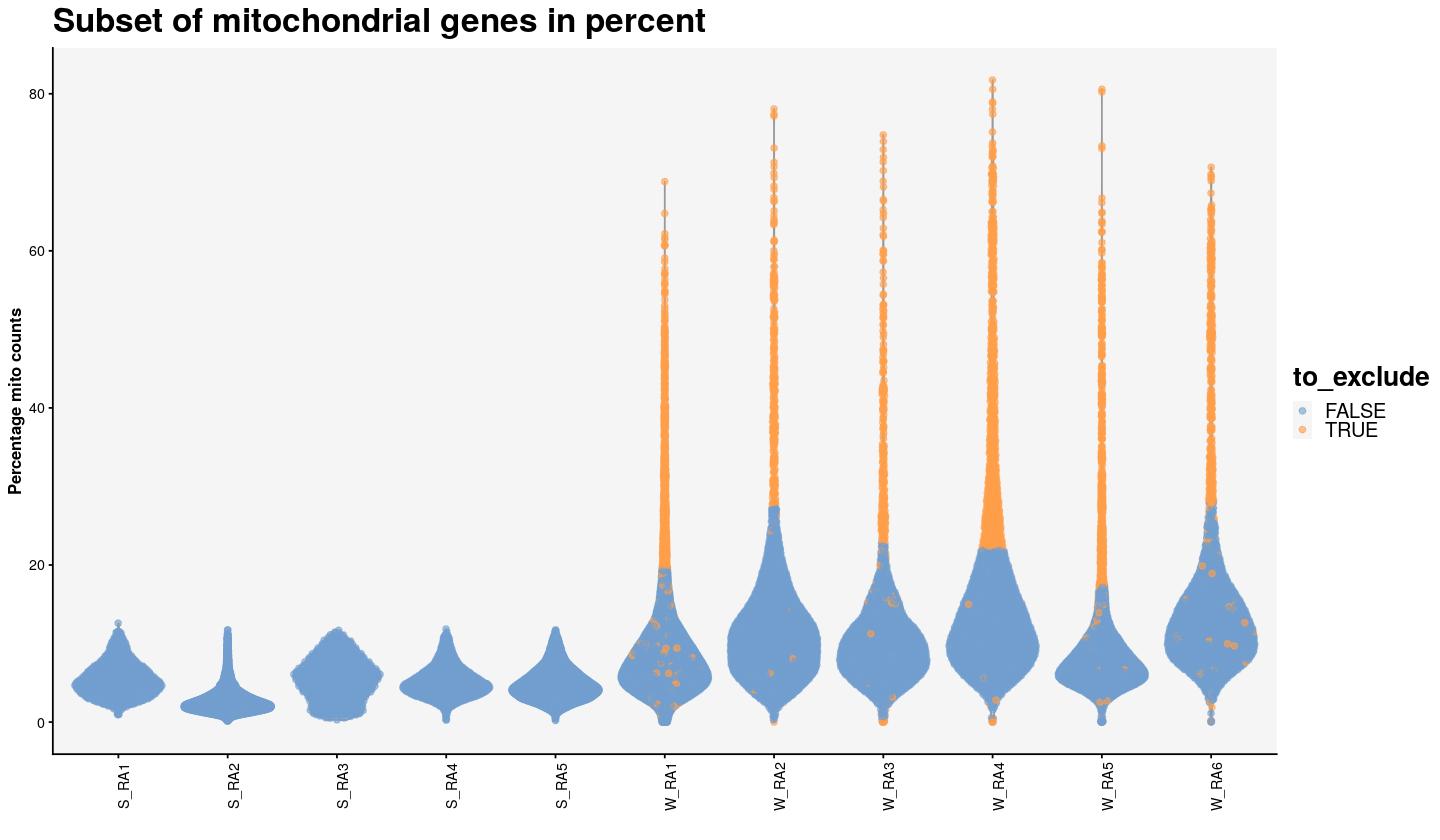
percentage mitochondrial counts per sample, each dot is a cell
cat("### Mito vs. Total {.tabset}\n\n")Mito vs. Total
cat("#### Color by exclude\n\n")Color by exclude
print(syn_sce %>%
  ggplot(aes(x=total, y=subsets_genes_detected, color=to_exclude)) +
    geom_point(size=0.5) +
    facet_wrap(~Sample, nrow=4) +
    labs(title = "Total gene expression count vs. number of detected genes",
         x = "Total counts", y = "Number of genes",
         colour = "Exclude cell") +
    scale_x_log10() +
    scale_y_log10() +
    geom_density_2d(colour="black", alpha=0.5) +
    main_plot_theme())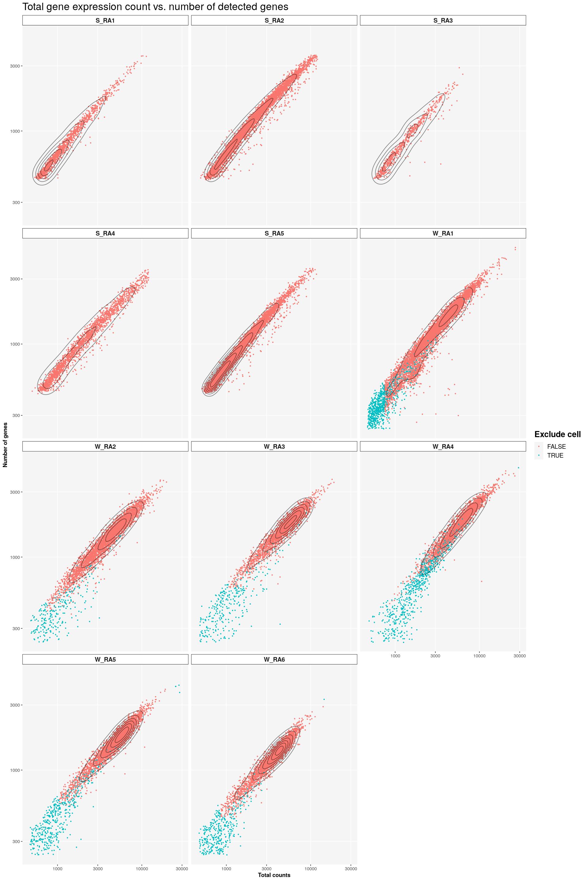
cat("\n\n")cat("#### Color by Mito\n\n")Color by Mito
print(syn_sce %>%
  ggplot(aes(x=total, y=subsets_genes_detected, color=subsets_Mito_percent)) +
    scale_color_gradient(low = "yellow", high = "darkred") +
    geom_point(size=0.5) +
    facet_wrap(~Sample, nrow=4) +
    labs(title = "Total gene expression count vs. number of detected genes",
       x = "Total counts", y = "Number of genes",
       colour = "Percentage\nMitochondrial\ncounts") +
    scale_x_log10() +
    scale_y_log10() +
    geom_density_2d(colour="black", alpha=0.5) +
    main_plot_theme())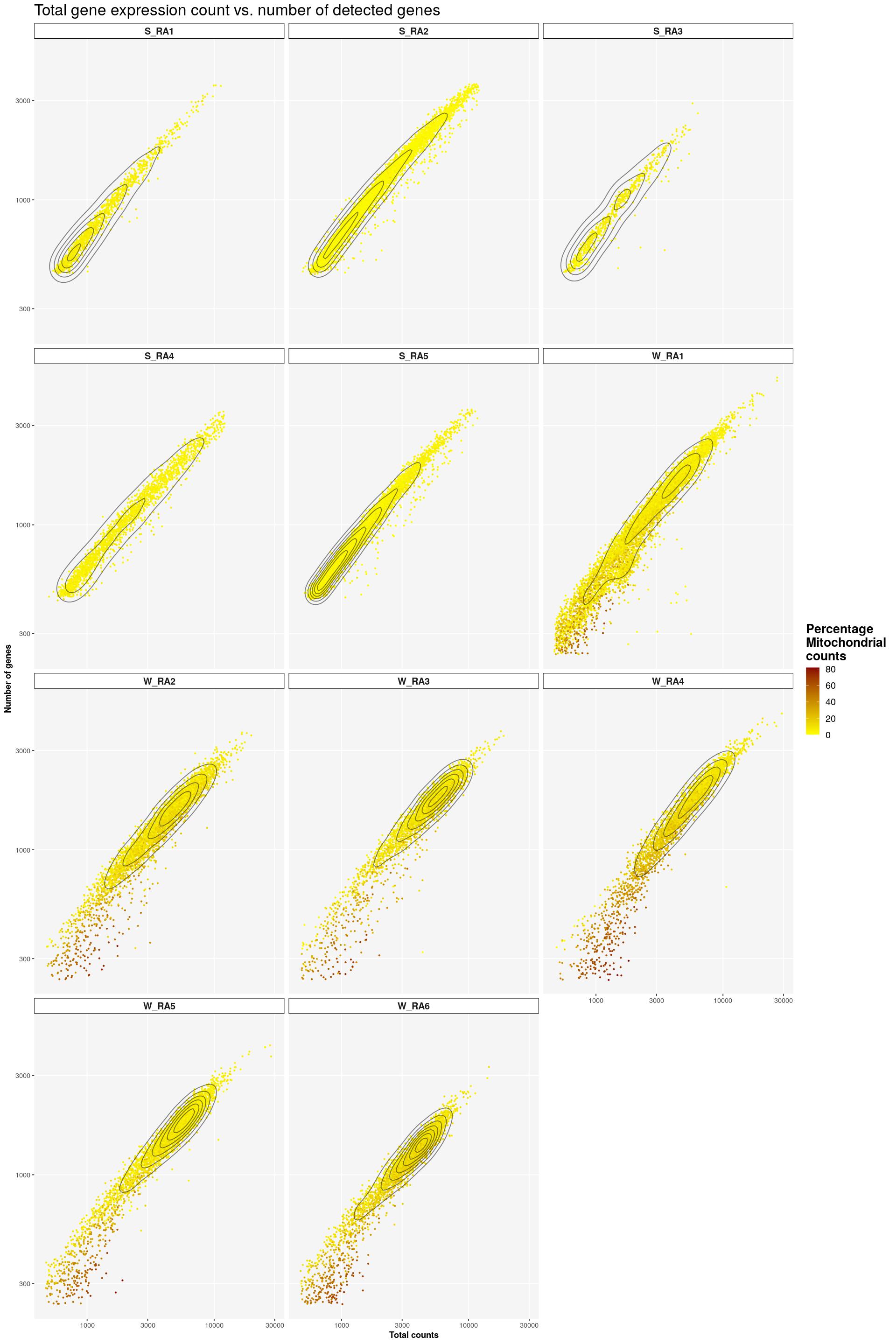
cat("\n\n")cat("### {-}")syn_sce %>%
plotColData(x=I(log(colData(syn_sce)$total)),
y="subsets_Mito_percent",
colour_by="to_exclude",
point_size=0.5,
point_alpha=0.5) +
ggtitle("Total gene expression values vs Total mitochondrial gene expression values") +
labs(x="log(Total counts)", y="Percentage mito counts") +
facet_wrap(~syn_sce$Sample, nrow = 5) +
main_plot_theme() +
theme(legend.position = c(0.92,0.97), legend.background = element_rect(color="grey",fill = "white"), legend.margin = margin(10,10,10,10))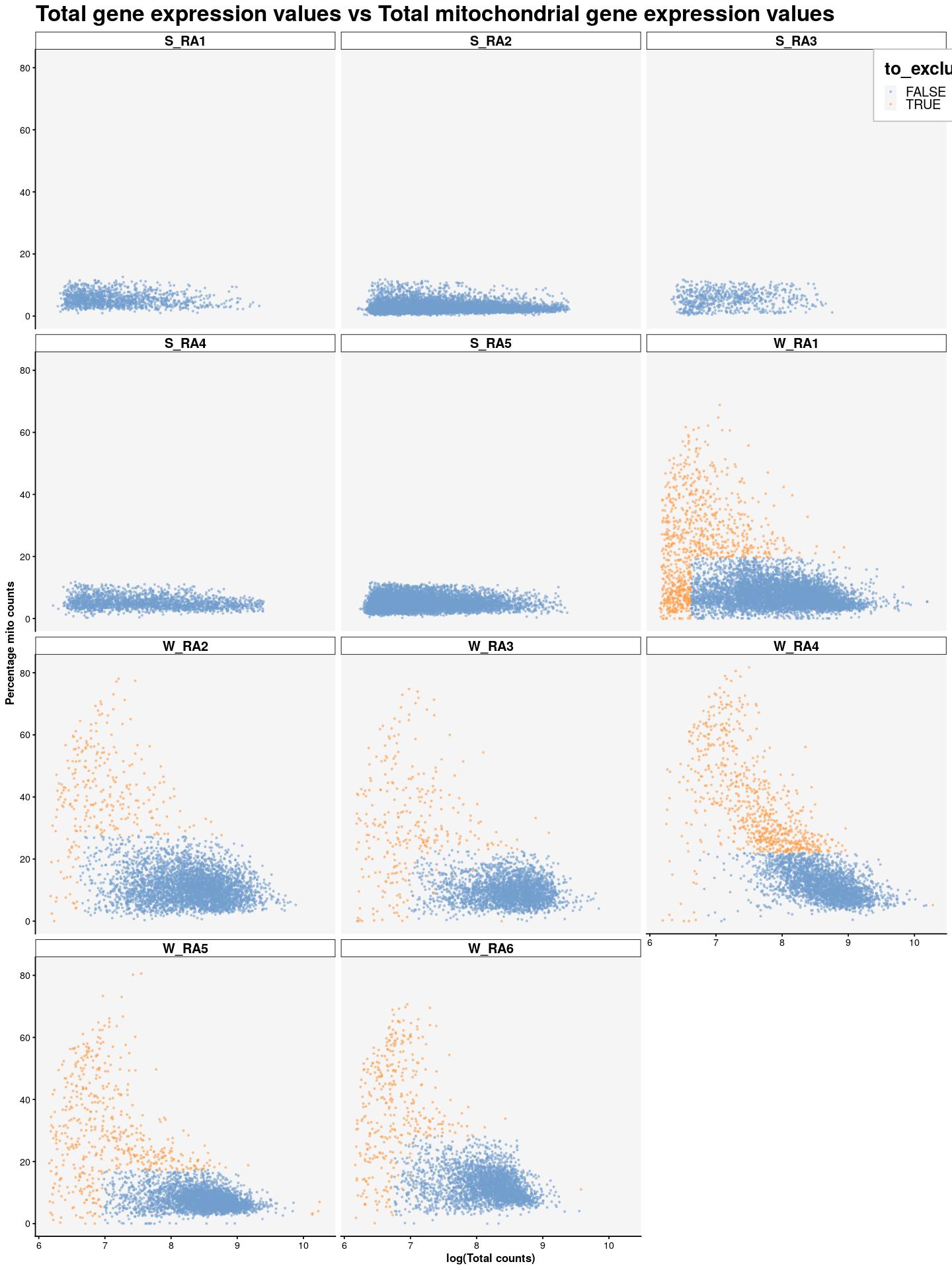
SampleQC
Another cell quality method, called SampleQC.
library(SampleQC)Bioconductor version '3.12' is out-of-date; the current release version '3.16'
is available with R version '4.2'; see https://bioconductor.org/installsyn_sce$patient_id <- syn_sce$Sample
syn_sce$sample_id <- syn_sce$Sample
rownames(syn_sce) <- rowData(syn_sce)$Symbol
qc_dt = suppressWarnings(make_qc_dt(syn_sce))
qc_names = c('log_counts', 'log_feats', 'logit_mito')
annots_disc = c('patient_id')
annots_cont = NULL
tmp <- capture.output(qc_obj <-
calc_pairwise_mmds(qc_dt,
qc_names,
annots_disc=annots_disc,
annots_cont=annots_cont,
n_cores=n_workers,
seed = 123)
)sample-level parts of SampleQC: calculating 55 sample-sample MMDs: clustering samples using MMD values calculating MDS embedding calculating UMAP embedding adding annotation variables constructing SampleQC objecttmp <- capture.output(qc_obj <-
fit_sampleqc(qc_obj,
K_list=rep(1, get_n_groups(qc_obj)),
bp_seed = 123)
)max 50 EM iterations:
.
took 1 iterationsmax 50 EM iterations:
.
took 1 iterationsoutliers_dt = get_outliers(qc_obj)
# sort and add
colData(syn_sce)$SampleQC_outlier[match(outliers_dt$cell_id, colnames(syn_sce))] <- outliers_dt$outlier
syn_sce <- syn_sce %>%
dplyr::mutate(SampleQC_outlier_mito =
(syn_sce$SampleQC_outlier | syn_sce$high_mitochondrion | syn_sce$total_counts_drop_fix) &
(syn_sce$Protocol != "stephenson"))
# comparison to scuttle
table(scuttle=syn_sce$to_exclude, SampleQC=syn_sce$SampleQC_outlier) SampleQC
scuttle FALSE TRUE
FALSE 37744 2936
TRUE 976 2072# comparison to scuttle, add mito limit to SampleQC
table(scuttle=syn_sce$to_exclude, SampleQC=syn_sce$SampleQC_outlier_mito) SampleQC
scuttle FALSE TRUE
FALSE 39064 1616
TRUE 1 3047syn_sce %>%
plotColData(x="Sample", y="subsets_Mito_percent", colour_by="SampleQC_outlier_mito") +
labs(x="", y="Percentage mito counts")+
theme(axis.text.x = element_text(angle = 90)) +
ggtitle("Subset of mitochondrial genes in percent") +
main_plot_theme() 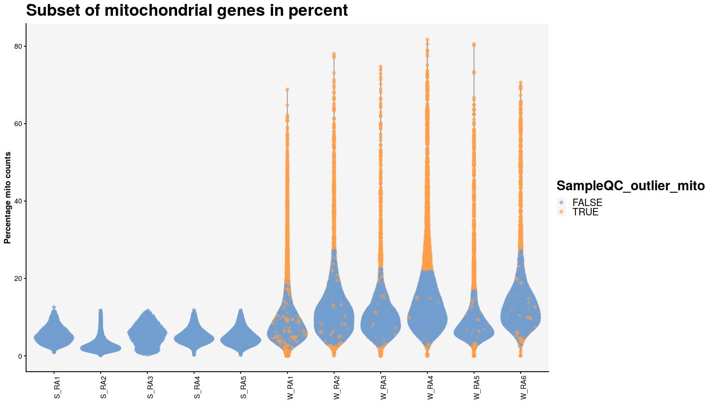
cat("### Mito vs. Total {.tabset}\n\n")Mito vs. Total
cat("#### Color by exclude\n\n")Color by exclude
sfig1a1 <- syn_sce %>%
  dplyr::select(total, subsets_genes_detected, SampleQC_outlier_mito, Sample) %>%
  ggplot(aes(x=total, y=subsets_genes_detected, color=SampleQC_outlier_mito)) +
    geom_point(size=0.5) +
    facet_wrap(~Sample, nrow=4) +
    labs(title = "Total gene expression count vs. number of detected genes",
         x = "Total counts", y = "Number of genes",
         colour = "Exclude cell") +
    scale_x_log10() +
    scale_y_log10() +
    geom_density_2d(colour="black", alpha=0.5) +
    main_plot_theme()
tidySingleCellExperiment says: Key columns are missing. A data frame is returned for independent data analysis.print(sfig1a1)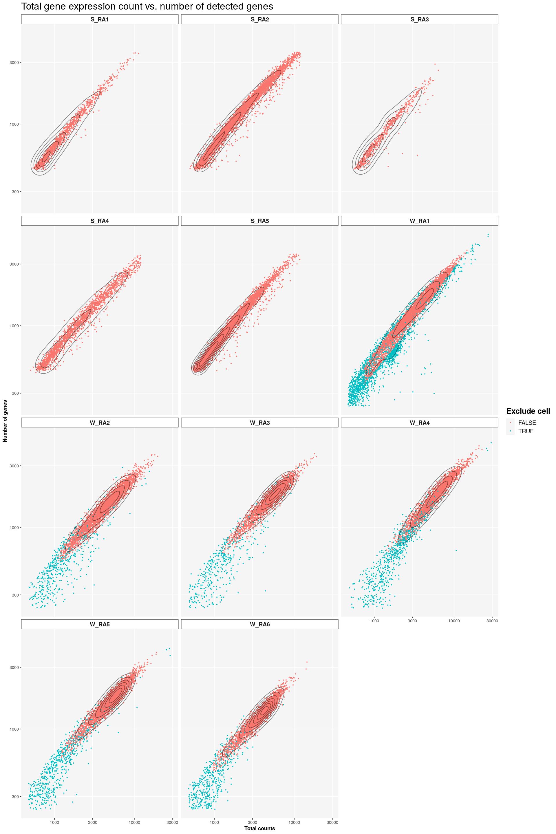
cat("\n\n")cat("#### Color by Mito\n\n")Color by Mito
sfig1a2 <- syn_sce %>%
  dplyr::select(total, subsets_genes_detected, subsets_Mito_percent, Sample) %>%
  ggplot(aes(x=total, y=subsets_genes_detected, color=subsets_Mito_percent)) +
    scale_color_gradient(low = "yellow", high = "darkred") +
    geom_point(size=0.5) +
    facet_wrap(~Sample, nrow=4) +
    labs(title = "Total gene expression count vs. number of detected genes",
       x = "Total counts", y = "Number of genes",
       colour = "Percentage\nMitochondrial\ncounts") +
    scale_x_log10() +
    scale_y_log10() +
    geom_density_2d(colour="black", alpha=0.5) +
    main_plot_theme()
tidySingleCellExperiment says: Key columns are missing. A data frame is returned for independent data analysis.print(sfig1a2)
cat("\n\n")cat("### {-}")syn_sce %>%
plotColData(x=I(log(colData(syn_sce)$total)),
y="subsets_Mito_percent",
colour_by="SampleQC_outlier_mito",
point_size=0.5,
point_alpha=0.5) +
ggtitle("Total gene expression values vs Total mitochondrial gene expression values") +
labs(x="log(Total counts)", y="Percentage mito counts") +
facet_wrap(~syn_sce$Sample, nrow = 5) +
main_plot_theme() +
theme(legend.position = c(0.92,0.97), legend.background = element_rect(color="grey",fill = "white"), legend.margin = margin(10,10,10,10))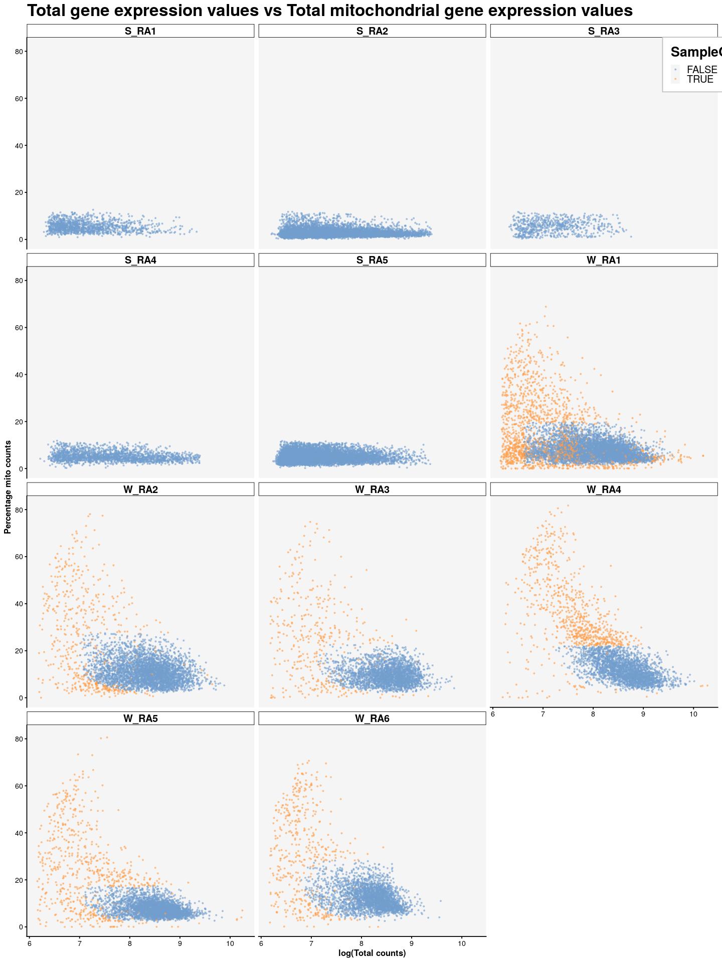
dim(syn_sce)[1] 14170 43728syn_sce_filtered <- syn_sce %>% filter(!SampleQC_outlier_mito)
dim(syn_sce_filtered)[1] 14170 39065syn_sce_filtered <- syn_sce_filtered[rowSums(counts(syn_sce_filtered) > 0) > 10, ]
dim(syn_sce_filtered)[1] 14170 39065prepare abundance plot data.
syn_nest_Sample <- syn_sce_filtered %>%
  nest(data=-Sample) %>%
  mutate(n_cells = purrr::map_dbl(data, ~ dim(.x)[2]),
         n_nonzero_genes = purrr::map_dbl(data, ~ sum(rowSums(counts(.x) > 0) > 0)),
         n_10cells_genes = purrr::map_dbl(data, ~ sum(rowSums(counts(.x) > 0) > 10)),
         n_1perc_cells_genes = purrr::map_dbl(data, ~ sum(rowSums(counts(.x) > 0) > ceiling(dim(.x)[2]/100))))

syn_nest_protocol <- syn_sce_filtered %>%
  nest(data=-Protocol) %>%
  mutate(n_cells = purrr::map_dbl(data, ~ dim(.x)[2]),
         n_nonzero_genes = purrr::map_dbl(data, ~ sum(rowSums(counts(.x) > 0) > 0)),
         n_10cells_genes = purrr::map_dbl(data, ~ sum(rowSums(counts(.x) > 0) > 10)),
         n_1perc_cells_genes = purrr::map_dbl(data, ~ sum(rowSums(counts(.x) > 0) > ceiling(dim(.x)[2]/100))))
plot abundances, colored by number of genes detected.
cat("### Number of Cells {.tabset}\n\n")Number of Cells
cat("#### Unique Samples \n\n")Unique Samples
sfig1b1 <- ggpubr::ggarrange(
  ggplot(syn_nest_Sample, aes(x = Sample, y = n_cells, fill = n_nonzero_genes)) +  # Plot with values on top
    geom_bar(stat = "identity") +
    geom_text(aes(label = n_cells), vjust = 0) +
    labs(title = "", x="", fill="Number of genes", y="Number of cells") +
  main_plot_theme() +
    theme(axis.text.x = element_text(angle = 45,hjust=1), axis.ticks.x=element_blank(),
          legend.position = c(1.1,0.5),plot.margin = margin(0,110,0,0)),
  ggplot(syn_nest_Sample, aes(x = Sample, y = n_cells, fill = n_1perc_cells_genes)) +  # Plot with values on top
    geom_bar(stat = "identity") +
    geom_text(aes(label = n_cells), vjust = 0) +
    labs(title = "", x="",
         fill="Number of genes\nin at least \n1% of cells",  y="Number of cells") +
    theme(axis.text.x = element_text(angle = 45,hjust=1), axis.ticks.x=element_blank(),
          legend.position = c(1.1,0.5),plot.margin = margin(0,110,0,0)) +
  main_plot_theme(),
  nrow = 2)
print(sfig1b1)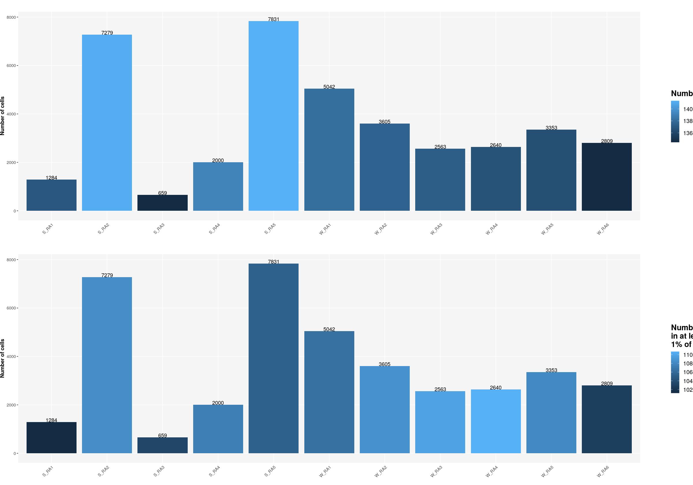
cat("\n\n")cat("#### Protocol \n\n")Protocol
sfig1b2 <- ggpubr::ggarrange(
  ggplot(syn_nest_protocol, aes(x = Protocol, y = n_cells, fill = n_nonzero_genes)) +  # Plot with values on top
    geom_bar(stat = "identity") +
    geom_text(aes(label = n_cells), vjust = 0) +
    labs(title = "", x="", fill="Number of genes", y="Number of cells") +
  main_plot_theme() +
    theme(axis.text.x = element_text(angle = 45,hjust=1), axis.ticks.x=element_blank(),
          legend.position = c(1.1,0.5),plot.margin = margin(0,110,0,0)),
  ggplot(syn_nest_protocol, aes(x = Protocol, y = n_cells, fill = n_1perc_cells_genes)) +  # Plot with values on top
    geom_bar(stat = "identity") +
    geom_text(aes(label = n_cells), vjust = 0) +
    labs(title = "", x="",
         fill="Number of genes\nin at least \n1% of cells",  y="Number of cells") +
    theme(axis.text.x = element_text(angle = 45,hjust=1), axis.ticks.x=element_blank(),
          legend.position = c(1.1,0.5),plot.margin = margin(0,110,0,0)) +
  main_plot_theme(),
  nrow = 2)
print(sfig1b2)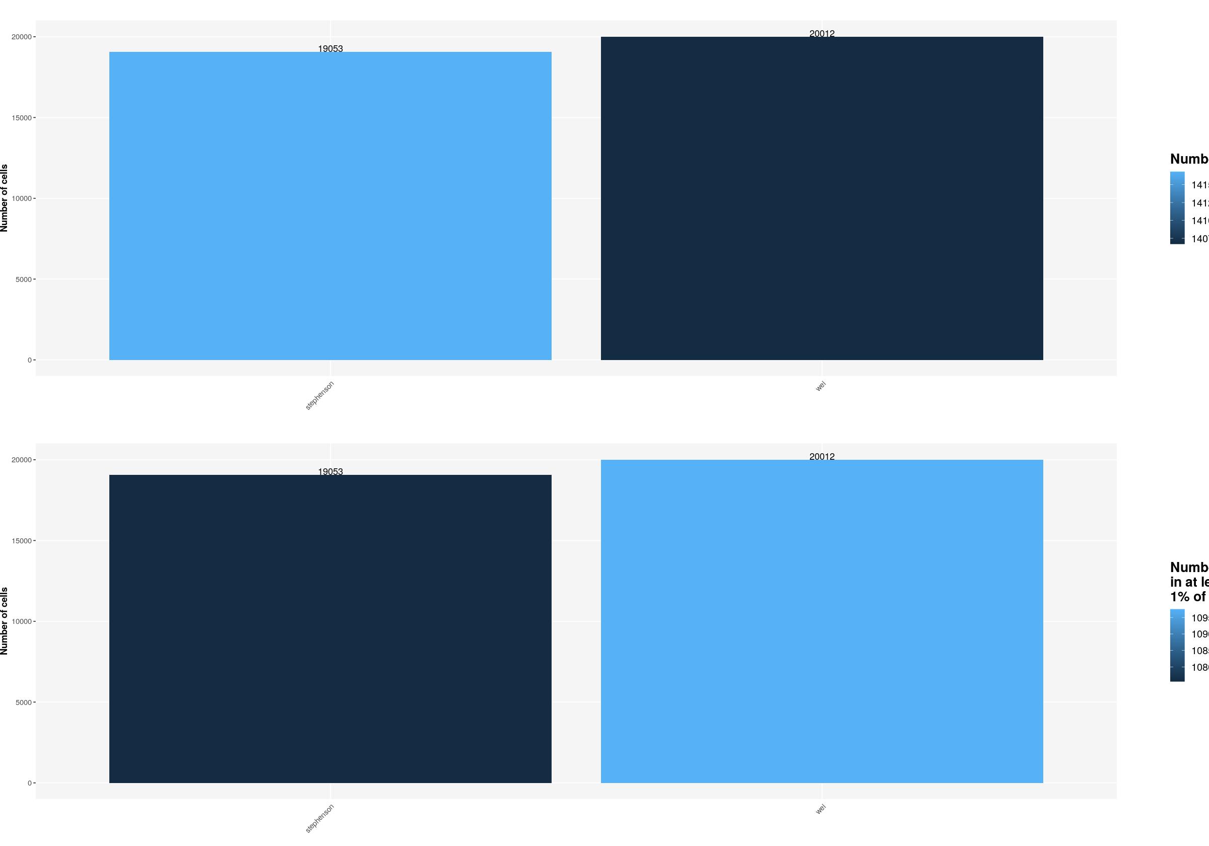
cat("\n\n")cat("### {-}")Normalization
Histogram of library size factors. Also quick clustering and computation of sum factors for better normalization (i.e. corrected for variability between celltypes).
set.seed(123)
bpstart(bpparam)
syn_sce_filtered$librarySizeFactors <- syn_sce_filtered %>%  librarySizeFactors(BPPARAM=bpparam)
bpstop(bpparam)
hist(log10(syn_sce_filtered$librarySizeFactors), xlab="Log10[Size factor]", col='grey80')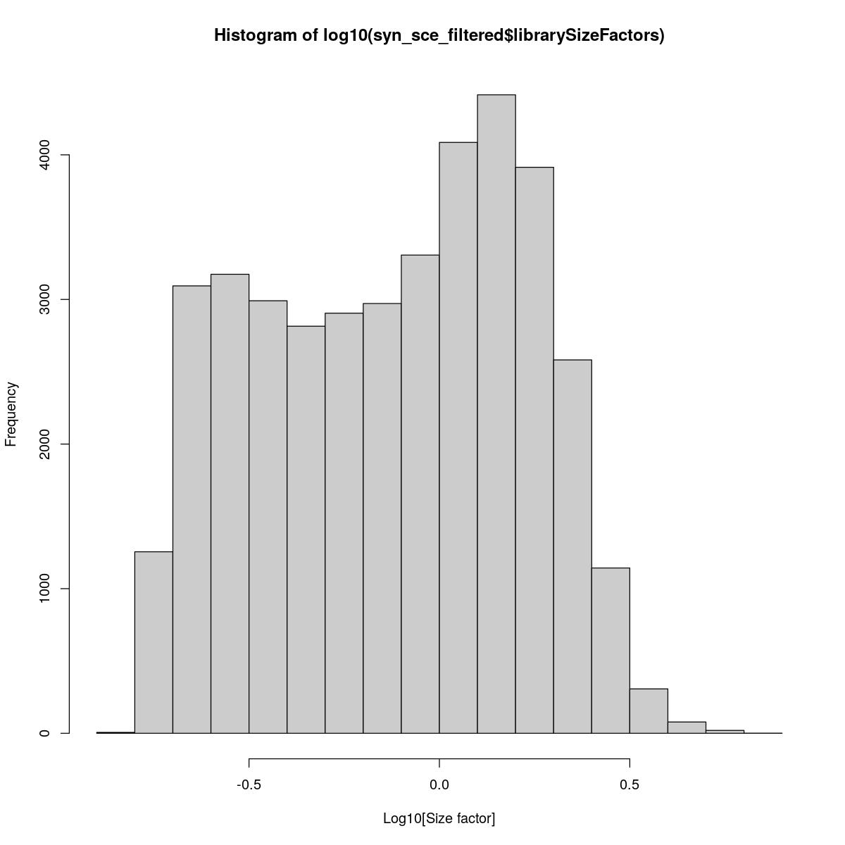
bpstart(bpparam)
clust.sce <- syn_sce_filtered %>%  quickCluster(BPPARAM=bpparam, block=factor(syn_sce_filtered$Protocol))
Warning in regularize.values(x, y, ties, missing(ties), na.rm = na.rm):
collapsing to unique 'x' valuesbpstop(bpparam)
bpstart(bpparam)
syn_sce_filtered <- syn_sce_filtered %>% computeSumFactors(clusters=clust.sce, BPPARAM=bpparam)
bpstop(bpparam)set.seed(1234)
ransam <- sample(seq_along(sizeFactors(syn_sce_filtered)))
plot(syn_sce_filtered$librarySizeFactors[ransam], sizeFactors(syn_sce_filtered)[ransam], xlab="Library size factor",
ylab="Deconvolution size factor", log='xy', pch=16,
col=as.integer(factor(clust.sce))[ransam],
main="Deconvolution factors for individual cluster")
abline(a=0, b=1, col="red")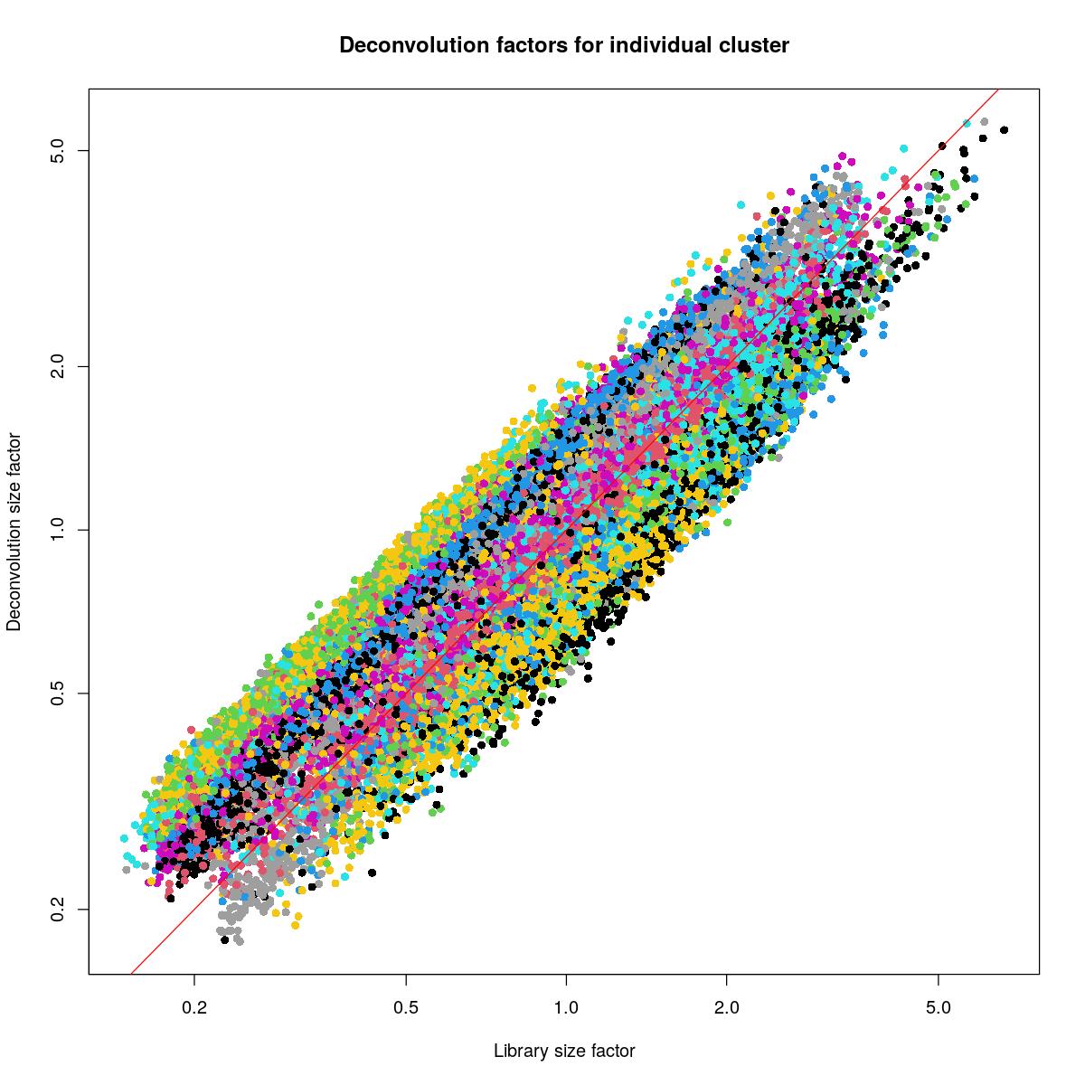
plot(syn_sce_filtered$librarySizeFactors[ransam], sizeFactors(syn_sce_filtered)[ransam], xlab="Library size factor",
    ylab="Deconvolution size factor", log='xy', pch=16,
    col=as.integer(factor(syn_sce_filtered$Sample))[ransam],
    main="Deconvolution factors for individual Sample")
abline(a=0, b=1, col="red")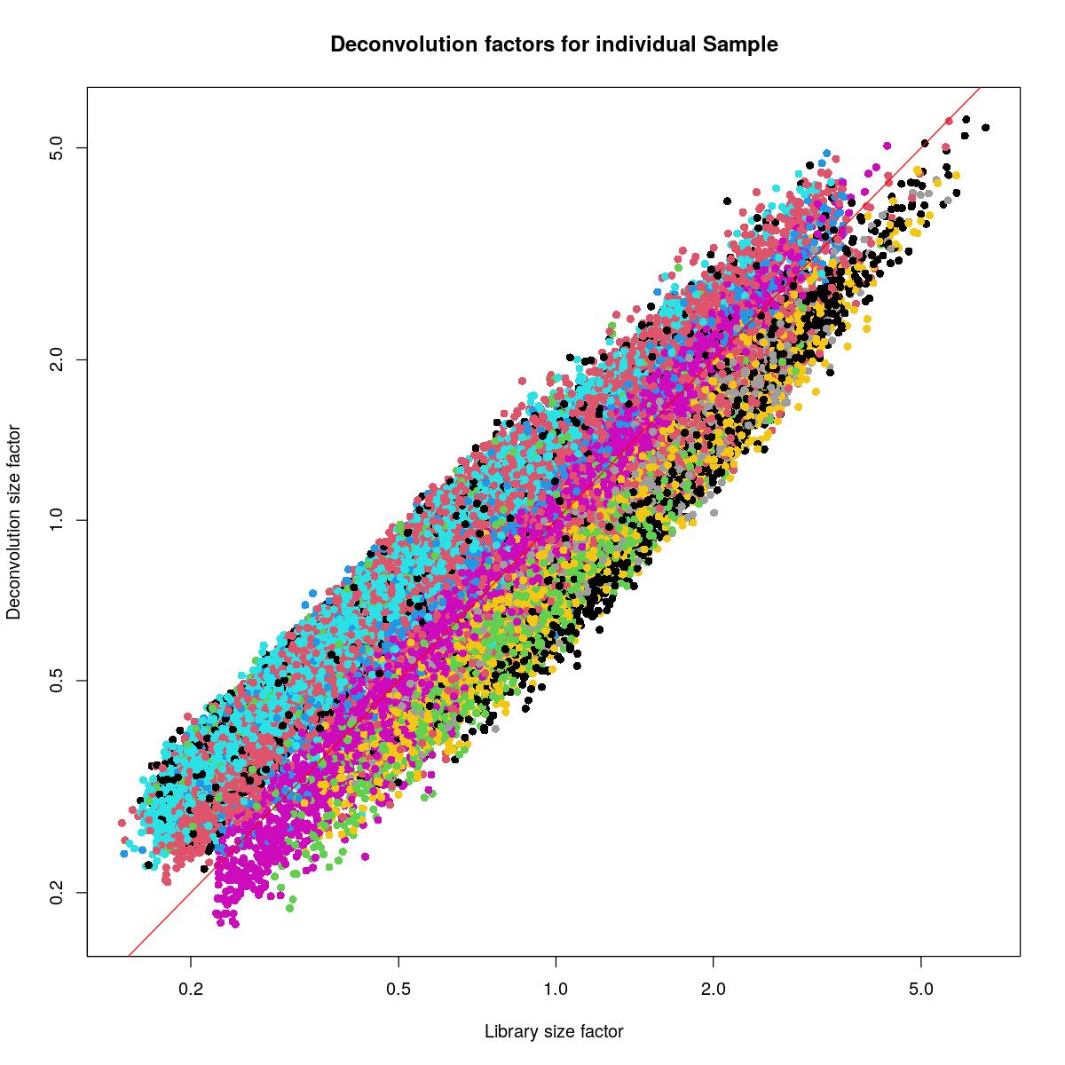
plot(syn_sce_filtered$librarySizeFactors[ransam], sizeFactors(syn_sce_filtered)[ransam], xlab="Library size factor",
    ylab="Deconvolution size factor", log='xy', pch=16,
    col=as.integer(factor(syn_sce_filtered$Protocol))[ransam],
    main="Deconvolution factors for individual Protocol")
abline(a=0, b=1, col="red")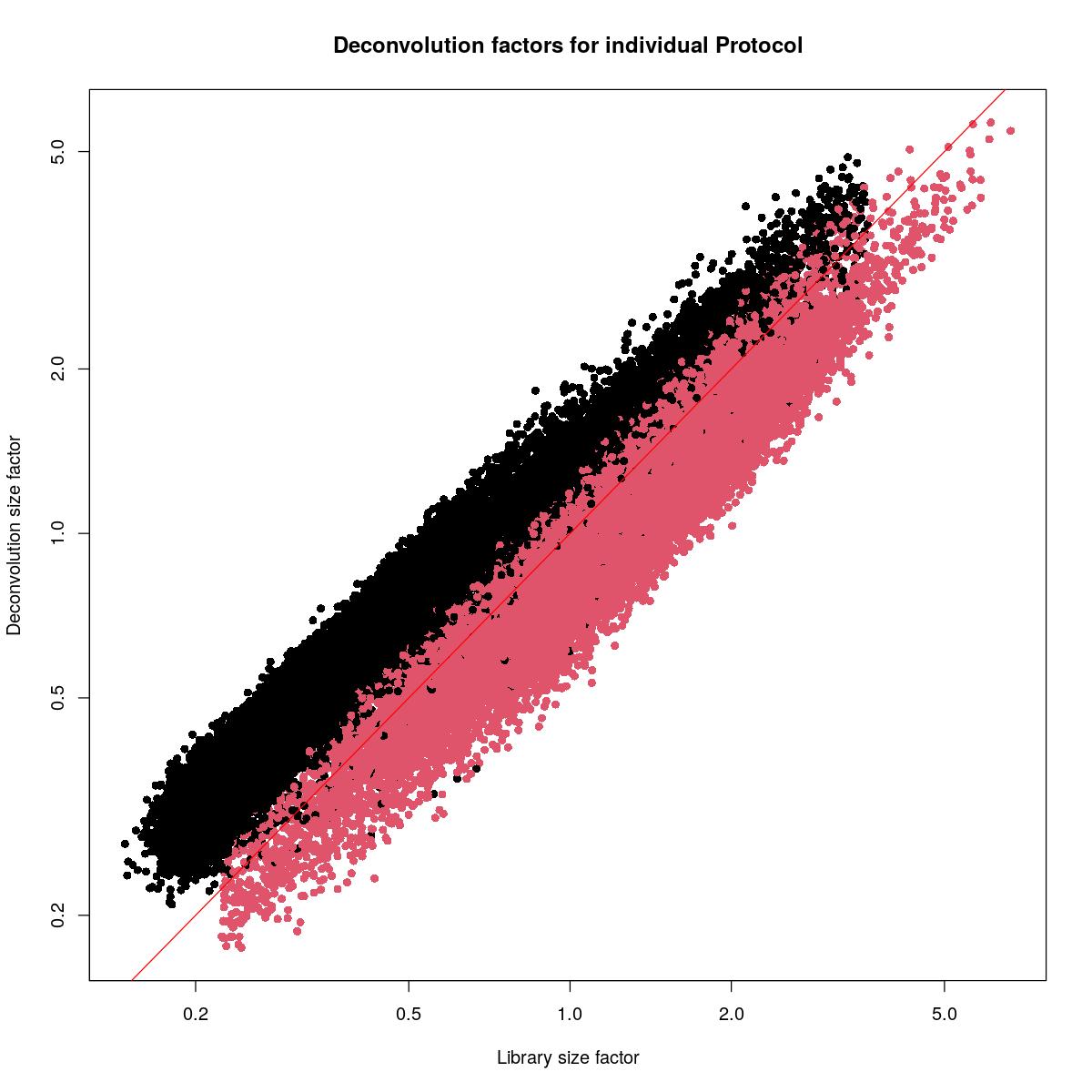
Apply normalization, run PCA.
set.seed(123)
syn_sce_filtered <- syn_sce_filtered %>%
  logNormCounts() %>%
  # logNormCounts(size.factors=syn_sce_filtered$librarySizeFactors, name="logcounts_librarySizeFactors") %>%
  runPCA()
size_fac_for_plotting <- I(librarySizeFactors(syn_sce_filtered))
table(factor(size_fac_for_plotting > 3, labels = c("<= 3", "> 3")))/length(size_fac_for_plotting)
     <= 3       > 3
0.9858953 0.0141047
size_fac_for_plotting[size_fac_for_plotting > 3] <- 3
plotPCA(syn_sce_filtered, colour_by=size_fac_for_plotting, ncomponents=2) + ggtitle(paste("Size factors"))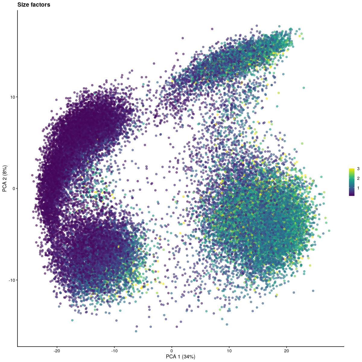
plot PCA, colored by size factor.
pca_pl_ls <- list()
for(pa_id in unique(syn_sce_filtered$patient_ID)){
  pat_filt <- syn_sce_filtered$patient_ID==pa_id
  pca_pl_ls[[pa_id]] <- plotPCA(syn_sce_filtered %>% filter(pat_filt), colour_by=size_fac_for_plotting[pat_filt], ncomponents=2) + ggtitle(paste("Size factor for Patient:",pa_id))
}
n_sam <- length(pca_pl_ls)
cat("### By Patient {.tabset}\n\n")
By Patient
for(i in seq_len(ceiling(n_sam/4))){
  pl_ind <- (((i-1)*4)+1):(((i)*4))
  pl_ind <- pl_ind[pl_ind <= n_sam]
  if(length(pl_ind) > 0){
    cat("#### Patients: ",paste(names(pca_pl_ls)[pl_ind]),"\n\n")
    print(ggpubr::ggarrange(plotlist=pca_pl_ls[pl_ind]))
    cat("\n\n")
  }
}
cat("### {-}")
saveRDS(syn_sce_filtered, file = here::here("output",paste0("combined_v",analysis_version,"_sce_filtered.rds")))
sessionInfo()R version 4.0.3 (2020-10-10)
Platform: x86_64-pc-linux-gnu (64-bit)
Running under: Ubuntu 20.04 LTS
Matrix products: default
BLAS/LAPACK: /usr/lib/x86_64-linux-gnu/openblas-pthread/libopenblasp-r0.3.8.so
locale:
[1] LC_CTYPE=en_US.UTF-8 LC_NUMERIC=C
[3] LC_TIME=en_US.UTF-8 LC_COLLATE=en_US.UTF-8
[5] LC_MONETARY=en_US.UTF-8 LC_MESSAGES=C
[7] LC_PAPER=en_US.UTF-8 LC_NAME=C
[9] LC_ADDRESS=C LC_TELEPHONE=C
[11] LC_MEASUREMENT=en_US.UTF-8 LC_IDENTIFICATION=C
attached base packages:
[1] parallel stats4 stats graphics grDevices utils datasets
[8] methods base
other attached packages:
[1] SampleQC_0.6.0 gdtools_0.2.3
[3] BiocParallel_1.24.1 tidySingleCellExperiment_1.0.0
[5] scuttle_1.0.4 scran_1.18.7
[7] scater_1.18.6 ggplot2_3.3.3
[9] SingleCellExperiment_1.12.0 SummarizedExperiment_1.20.0
[11] Biobase_2.50.0 GenomicRanges_1.42.0
[13] GenomeInfoDb_1.26.7 IRanges_2.24.1
[15] S4Vectors_0.28.1 BiocGenerics_0.36.1
[17] MatrixGenerics_1.2.1 matrixStats_0.58.0
[19] purrr_0.3.4 dplyr_1.0.4
[21] workflowr_1.6.2
loaded via a namespace (and not attached):
[1] readxl_1.3.1 backports_1.2.1
[3] systemfonts_1.0.1 igraph_1.2.6
[5] lazyeval_0.2.2 splines_4.0.3
[7] digest_0.6.27 htmltools_0.5.1.1
[9] viridis_0.5.1 fansi_0.4.2
[11] magrittr_2.0.1 mixtools_1.2.0
[13] openxlsx_4.2.3 limma_3.46.0
[15] svglite_1.2.3.2 colorspace_2.0-0
[17] haven_2.3.1 xfun_0.21
[19] crayon_1.4.1 RCurl_1.98-1.2
[21] jsonlite_1.7.2 survival_3.2-7
[23] glue_1.4.2 gtable_0.3.0
[25] zlibbioc_1.36.0 XVector_0.30.0
[27] DelayedArray_0.16.3 car_3.0-10
[29] BiocSingular_1.6.0 kernlab_0.9-29
[31] abind_1.4-5 scales_1.1.1
[33] mvtnorm_1.1-1 DBI_1.1.1
[35] edgeR_3.32.1 rstatix_0.7.0
[37] Rcpp_1.0.6 isoband_0.2.3
[39] viridisLite_0.3.0 dqrng_0.2.1
[41] foreign_0.8-81 rsvd_1.0.3
[43] mclust_5.4.7 htmlwidgets_1.5.3
[45] httr_1.4.2 RColorBrewer_1.1-2
[47] ellipsis_0.3.1 pkgconfig_2.0.3
[49] farver_2.0.3 uwot_0.1.10
[51] locfit_1.5-9.4 here_1.0.1
[53] tidyselect_1.1.0 labeling_0.4.2
[55] rlang_0.4.10 later_1.1.0.1
[57] cellranger_1.1.0 munsell_0.5.0
[59] tools_4.0.3 cli_2.3.0
[61] generics_0.1.0 broom_0.7.4
[63] evaluate_0.14 stringr_1.4.0
[65] yaml_2.2.1 RhpcBLASctl_0.20-137
[67] knitr_1.31 fs_1.5.0
[69] zip_2.1.1 sparseMatrixStats_1.2.1
[71] mvnfast_0.2.5.1 BiocStyle_2.18.1
[73] compiler_4.0.3 beeswarm_0.2.3
[75] plotly_4.9.3 curl_4.3
[77] ggsignif_0.6.0 tibble_3.0.6
[79] statmod_1.4.35 stringi_1.5.3
[81] highr_0.8 RSpectra_0.16-0
[83] forcats_0.5.1 lattice_0.20-41
[85] bluster_1.0.0 Matrix_1.3-2
[87] vctrs_0.3.6 pillar_1.4.7
[89] lifecycle_1.0.0 BiocManager_1.30.12
[91] BiocNeighbors_1.8.2 data.table_1.13.6
[93] cowplot_1.1.1 bitops_1.0-6
[95] irlba_2.3.3 httpuv_1.5.5
[97] patchwork_1.1.1 R6_2.5.0
[99] promises_1.2.0.1 gridExtra_2.3
[101] rio_0.5.16 vipor_0.4.5
[103] MASS_7.3-53.1 gtools_3.8.2
[105] assertthat_0.2.1 rprojroot_2.0.2
[107] withr_2.4.1 GenomeInfoDbData_1.2.4
[109] hms_1.0.0 grid_4.0.3
[111] beachmat_2.6.4 tidyr_1.1.2
[113] rmarkdown_2.6 DelayedMatrixStats_1.12.3
[115] carData_3.0-4 segmented_1.3-2
[117] git2r_0.28.0 ggpubr_0.4.0
[119] ggbeeswarm_0.6.0