scRNAseq_complete_00_ambient_RNA
retogerber
2022-10-18
Last updated: 2022-10-18
Checks: 6 1
Knit directory: synovialscrnaseq/
This reproducible R Markdown analysis was created with workflowr (version 1.6.2). The Checks tab describes the reproducibility checks that were applied when the results were created. The Past versions tab lists the development history.
The R Markdown file has unstaged changes. To know which version of the R Markdown file created these results, you’ll want to first commit it to the Git repo. If you’re still working on the analysis, you can ignore this warning. When you’re finished, you can run wflow_publish to commit the R Markdown file and build the HTML.
Great job! The global environment was empty. Objects defined in the global environment can affect the analysis in your R Markdown file in unknown ways. For reproduciblity it’s best to always run the code in an empty environment.
The command set.seed(20210105) was run prior to running the code in the R Markdown file. Setting a seed ensures that any results that rely on randomness, e.g. subsampling or permutations, are reproducible.
Great job! Recording the operating system, R version, and package versions is critical for reproducibility.
Nice! There were no cached chunks for this analysis, so you can be confident that you successfully produced the results during this run.
Great job! Using relative paths to the files within your workflowr project makes it easier to run your code on other machines.
Great! You are using Git for version control. Tracking code development and connecting the code version to the results is critical for reproducibility.
The results in this page were generated with repository version 816d5c9. See the Past versions tab to see a history of the changes made to the R Markdown and HTML files.
Note that you need to be careful to ensure that all relevant files for the analysis have been committed to Git prior to generating the results (you can use wflow_publish or wflow_git_commit). workflowr only checks the R Markdown file, but you know if there are other scripts or data files that it depends on. Below is the status of the Git repository when the results were generated:
Ignored files:
    Ignored:    '/
    Ignored:    .Rhistory
    Ignored:    .Rproj.user/
    Ignored:    .empty/
    Ignored:    analysis/.Rhistory
    Ignored:    analysis/iSEE_interactive_document.html
    Ignored:    code/test_files/
    Ignored:    data/Culemann/
    Ignored:    data/E-MTAB-8322/
    Ignored:    data/Synovial scRNA-seq samples - Sheet1.csv
    Ignored:    data/Zhang_top20_singlecell_cluster_markers_fromGithub.csv
    Ignored:    data/findMarkers_results.rds
    Ignored:    data/findMarkers_results_v2.rds
    Ignored:    data/info/
    Ignored:    data/syn_sce_tidy_filtered.rds
    Ignored:    data/syn_sce_tidy_hvg.rds
    Ignored:    data/syn_sce_tidy_hvg_cms.rds
    Ignored:    docs/
    Ignored:    output/Figures_Paper/
    Ignored:    output/Sample_summaries_RA_comparisons.rds
    Ignored:    output/Sample_summaries_direct_dissociation.rds
    Ignored:    output/Sample_summaries_exvivo_treatment.rds
    Ignored:    output/Suppl_Figure_4d.rds
    Ignored:    output/barcodes.txt
    Ignored:    output/count_matrix_unfiltered.mtx
    Ignored:    output/emptyDrops_result_v4_tmp.rds
    Ignored:    output/emptyDrops_result_v4tmptmp.rds
    Ignored:    output/entropies_fstat_v5_ec.rds
    Ignored:    output/entropies_fstat_v5_main.rds
    Ignored:    output/entropies_fstat_v5_mp.rds
    Ignored:    output/entropies_fstat_v5_sf.rds
    Ignored:    output/entropies_fstat_v5_tc.rds
    Ignored:    output/findMarkers_results_v5_ec.rds
    Ignored:    output/findMarkers_results_v5_main.rds
    Ignored:    output/findMarkers_results_v5_mp.rds
    Ignored:    output/findMarkers_results_v5_sf.rds
    Ignored:    output/findMarkers_results_v5_tc.rds
    Ignored:    output/findMarkers_results_v6.rds
    Ignored:    output/findMarkers_results_v6_ec.rds
    Ignored:    output/findMarkers_results_v6_main.rds
    Ignored:    output/findMarkers_results_v6_mp.rds
    Ignored:    output/findMarkers_results_v6_sf.rds
    Ignored:    output/findMarkers_results_v6_tc.rds
    Ignored:    output/genes.txt
    Ignored:    output/goana_results_v6_ec.rds
    Ignored:    output/goana_results_v6_mp.rds
    Ignored:    output/syn_v4_swappedDrops_24300_after.rds
    Ignored:    output/syn_v4_swappedDrops_24300_before.rds
    Ignored:    output/syn_v4_swappedDrops_24793_after.rds
    Ignored:    output/syn_v4_swappedDrops_24793_before.rds
    Ignored:    output/syn_v5_annot_df_manual.rds
    Ignored:    output/syn_v5_cluster_cellid_match_invivo.rds
    Ignored:    output/syn_v5_clustering_lookup_invivo.rds
    Ignored:    output/syn_v5_clustering_lookup_multiple_invivo.rds
    Ignored:    output/syn_v5_res_da_Accute_inflammation_invivo.rds
    Ignored:    output/syn_v5_res_da_Diagnosis_invivo.rds
    Ignored:    output/syn_v5_res_da_Diagnosis_main_invivo.rds
    Ignored:    output/syn_v5_res_da_Lymphoid_folicles_invivo.rds
    Ignored:    output/syn_v5_res_da_Pathotype_invivo.rds
    Ignored:    output/syn_v5_res_da_Therapy_invivo.rds
    Ignored:    output/syn_v5_res_da_Vascularisation_bin_invivo.rds
    Ignored:    output/syn_v5_res_ds_Accute_inflammation_invivo.rds
    Ignored:    output/syn_v5_res_ds_Diagnosis_invivo.rds
    Ignored:    output/syn_v5_res_ds_Diagnosis_main_invivo.rds
    Ignored:    output/syn_v5_res_ds_Lymphoid_folicles_invivo.rds
    Ignored:    output/syn_v5_res_ds_Pathotype_invivo.rds
    Ignored:    output/syn_v5_res_ds_Therapy_invivo.rds
    Ignored:    output/syn_v5_res_ds_Vascularisation_bin_invivo.rds
    Ignored:    output/syn_v5_sce.rds
    Ignored:    output/syn_v5_sce_ec_invivo.rds
    Ignored:    output/syn_v5_sce_filtered_invivo.rds
    Ignored:    output/syn_v5_sce_hvg_cms_doublet_annot_manual_invivo.rds
    Ignored:    output/syn_v5_sce_hvg_cms_doublet_cmstest_invivo.rds
    Ignored:    output/syn_v5_sce_hvg_cms_doublet_invivo.rds
    Ignored:    output/syn_v5_sce_hvg_cms_doublet_subcluster_invivo.rds
    Ignored:    output/syn_v5_sce_hvg_invivo.rds
    Ignored:    output/syn_v5_sce_mp_invivo.rds
    Ignored:    output/syn_v5_sce_sf_invivo.rds
    Ignored:    output/syn_v5_sce_tc_invivo.rds
    Ignored:    output/syn_v5_vst_out_invivo.rds
    Ignored:    output/syn_v6_cluster_cellid_match_invivo.rds
    Ignored:    output/syn_v6_clustering_lookup_invivo.rds
    Ignored:    output/syn_v6_clustering_lookup_multiple_invivo.rds
    Ignored:    output/syn_v6_sce.rds
    Ignored:    output/syn_v6_sce_Figure8.rds
    Ignored:    output/syn_v6_sce_Figure8_dic_ls.rds
    Ignored:    output/syn_v6_sce_ec_invivo.rds
    Ignored:    output/syn_v6_sce_filtered_invivo.rds
    Ignored:    output/syn_v6_sce_hdf5/
    Ignored:    output/syn_v6_sce_hvg_cms_doublet_invivo.rds
    Ignored:    output/syn_v6_sce_hvg_cms_doublet_subcluster_invivo.rds
    Ignored:    output/syn_v6_sce_hvg_invivo.rds
    Ignored:    output/syn_v6_sce_hvg_marker_genes.rds
    Ignored:    output/syn_v6_sce_mp_invivo.rds
    Ignored:    output/syn_v6_sce_sf_invivo.rds
    Ignored:    output/syn_v6_sce_tc_invivo.rds
    Ignored:    output/syn_v6_sfig1.rds
    Ignored:    output/syn_v6_vst_out_invivo.rds

Untracked files:
    Untracked:  analysis/22
    Untracked:  analysis/scRNAseq_complete_01_preprocessing_comparison.Rmd
    Untracked:  analysis/test.Rmd
    Untracked:  code/rebuild_ezRun.R
    Untracked:  nonhosted_public/
    Untracked:  singRstudio.sh.bak

Unstaged changes:
    Modified:   analysis/scRNAseq_complete_00_ambient_RNA.Rmd
    Modified:   analysis/scRNAseq_complete_Figures.Rmd
    Modified:   analysis/write_tsv.Rmd
Note that any generated files, e.g. HTML, png, CSS, etc., are not included in this status report because it is ok for generated content to have uncommitted changes.
These are the previous versions of the repository in which changes were made to the R Markdown (analysis/scRNAseq_complete_00_ambient_RNA.Rmd) and HTML (public/scRNAseq_complete_00_ambient_RNA.html) files. If you’ve configured a remote Git repository (see ?wflow_git_remote), click on the hyperlinks in the table below to view the files as they were in that past version.
| File | Version | Author | Date | Message |
|---|---|---|---|---|
| html | 3443cc6 | Reto Gerber | 2022-04-25 | Update |
| html | f2e34e1 | Reto Gerber | 2021-07-29 | Update navbar |
| Rmd | ee1face | Reto Gerber | 2021-07-29 | Add missing scripts |
| html | 222b0d1 | Reto Gerber | 2021-07-29 | Update analysis to v5 |
| Rmd | e88c23e | Reto Gerber | 2021-07-12 | add ambient RNA analysis |
| html | e88c23e | Reto Gerber | 2021-07-12 | add ambient RNA analysis |
| Rmd | 6b4ed06 | Reto Gerber | 2021-07-01 | Add new DS, update iSEE |
| Rmd | 83c0d88 | Reto Gerber | 2021-06-14 | bugfix iSEE_LandingPage.R |
| Rmd | 3072789 | Reto Gerber | 2021-06-09 | Update annotation scripts |
Set up
suppressPackageStartupMessages({
  library(dplyr)
  library(ggplot2)
  library(purrr)
  library(stringr)
  library(SummarizedExperiment)
  library(SingleCellExperiment)
  library(scater)
  library(scran)
  library(igraph)
  library(SingleR)
  library(scuttle)
  library(celldex)
  library(ggbeeswarm)
  library(tidySingleCellExperiment)
  library(bluster)
  library(DropletUtils)
  library(BiocParallel)
})
n_workers <- 10
RhpcBLASctl::blas_set_num_threads(n_workers)
bpparam <- MulticoreParam(workers = n_workers, RNGseed=123)
# bp_param <- BiocParallel::MulticoreParam(workers=20)

here::here()
[1] "/home/retger/Synovial/synovialscrnaseq"raw_data_dir <- here::here("..","data_server")
raw_data_dir_blaz <- here::here("..","data_blaz")
remove_low_quality_samples <- TRUE
set.seed(100)filter low quality samples
if(remove_low_quality_samples){
    samples_to_remove <- c("Syn_Bio_080","Syn_Bio_086","Syn_Bio_055_DMSO","Syn_Bio_055_Tofa","Syn_Bio_072_DMSO","Syn_Bio_072_Tofa","Syn_Bio_094_DMSO","Syn_Bio_094_Tofa")
#     samples_to_remove %in% syn_sce$Sample
# syn_sce <- syn_sce[,!(syn_sce$Sample %in% samples_to_remove)]
}
# prepare
samples <- here::here(raw_data_dir,list.files(raw_data_dir),"raw_feature_bc_matrix")
names(samples) <- purrr::map_chr(strsplit(samples, "/") , ~ .x[length(.x)-1])
samples_to_remove <- c("o23841_1_09-485", # Sample not belongin to Synovial
"o23841_1_13-26_10","26_10000","26_5000", # Aggregated into Aggr_26
"Aggr_26", # old (incorrect) version
"26_10_comb", # intermediate
"23_10000","23_5000", # Aggregated into Aggr_23
"31_10000","31_5000", # Aggregated into Aggr_31
"SynTissue_28_10000","SynTissue_28_5000", # Aggregated into Aggr_28
"o28599_SpaceRangerCount_2022-06-20--14-51-56" # new spatial data
)
samples <- samples[!stringr::str_detect(samples, paste0(samples_to_remove,collapse = "|"))]
sam_ind <- stringr::str_detect(samples,"Aggr_|26_comb")
samples[sam_ind] <- paste0(
purrr::map_chr(strsplit(samples[sam_ind], "/") , ~ paste0(.x[-length(.x)],collapse="/")),
"/outs/count/raw_feature_bc_matrix")metadata_df <- readRDS(here::here("output","Sample_summaries_direct_dissociation.rds"))
sce_swapped_ls <- list()
swappedDrops_samples_comb <- c()
rowdat_syn_sce <- DropletUtils::read10xCounts(samples=samples[20])
order_id <- "24300"# read swappedDrops data
after.mat <- readRDS(here::here("output",paste0("syn_v4_swappedDrops_",order_id,"_after.rds")))
swappedDrops_samples <- names(after.mat$cleaned)[names(after.mat$cleaned) %in% metadata_df$`FGCZ_Sample Name`]
if(remove_low_quality_samples){
swappedDrops_samples <- swappedDrops_samples[!(swappedDrops_samples %in% metadata_df$`FGCZ_Sample Name`[stringr::str_replace_all(metadata_df$Sample," ","_") %in% samples_to_remove])]
}
print(swappedDrops_samples)[1] "o24300_1_01-79" "o24300_1_02-86" "o24300_1_03-83" "o24300_1_04-84"
[5] "o24300_1_05-78" "o24300_1_06-81" "o24300_1_07-87" "o24300_1_11-80"
[9] "o24300_1_12-89"bpstart(bpparam)
sce_swapped_ls[[order_id]] <- BiocParallel::bplapply(BPPARAM = bpparam,
swappedDrops_samples,
function(i){
sce_tmp <- SingleCellExperiment(assays=SimpleList(counts=after.mat$cleaned[[i]]),
rowData=DataFrame(rowData(rowdat_syn_sce)),
colData=DataFrame(Sample=i,
Barcode=colnames(after.mat$cleaned[[i]]),
row.names=colnames(after.mat$cleaned[[i]]))
)
colData(sce_tmp) <- dplyr::left_join(as.data.frame(colData(sce_tmp)),
metadata_df,
by= c("Sample" = "FGCZ_Sample Name"),
suffix=c(".x",".y")) %>%
dplyr::rename(Sample_unique=Sample,
Sample=Sample.y) %>%
dplyr::mutate(Sample = dplyr::if_else(is.na(Sample), Sample_unique, Sample),
Sample = stringr::str_replace_all(Sample, " ", "_"),
Diagnosis = stringr::str_replace_all(Diagnosis, " ", "_")) %>%
DataFrame(row.names=colnames(sce_tmp))
colnames(sce_tmp) <- paste0(sce_tmp$Sample, ".", sce_tmp$Barcode)
rownames(sce_tmp) <- paste0(rowData(sce_tmp)$ID, ".", rowData(sce_tmp)$Symbol)
sce_tmp
})
bpstop(bpparam)
names(sce_swapped_ls[[order_id]]) <- swappedDrops_samples
swappedDrops_samples_comb <- c(swappedDrops_samples_comb,swappedDrops_samples)
rm(after.mat)
gc() used (Mb) gc trigger (Mb) max used (Mb)
Ncells 27965017 1493.5 59405312 3172.6 28346425 1513.9
Vcells 701041277 5348.6 1987275592 15161.8 2330557716 17780.8order_id <- "24793"# read swappedDrops data
after.mat <- readRDS(here::here("output",paste0("syn_v4_swappedDrops_",order_id,"_after.rds")))
swappedDrops_samples <- names(after.mat$cleaned)[names(after.mat$cleaned) %in% metadata_df$`FGCZ_Sample Name`]
if(remove_low_quality_samples){
swappedDrops_samples <- swappedDrops_samples[!(swappedDrops_samples %in% metadata_df$`FGCZ_Sample Name`[stringr::str_replace_all(metadata_df$Sample," ","_") %in% samples_to_remove])]
}
print(swappedDrops_samples)[1] "o24793_1_01-91" "o24793_1_02-92" "o24793_1_03-93" "o24793_1_04-95"
[5] "o24793_1_05-96" "o24793_1_06-98a" "o24793_1_07-98b" "o24793_1_08-99" bpstart(bpparam)
sce_swapped_ls[[order_id]] <- BiocParallel::bplapply(BPPARAM = bpparam,
swappedDrops_samples,
function(i){
sce_tmp <- SingleCellExperiment(assays=SimpleList(counts=after.mat$cleaned[[i]]),
rowData=DataFrame(rowData(rowdat_syn_sce)),
colData=DataFrame(Sample=i,
Barcode=colnames(after.mat$cleaned[[i]]),
row.names=colnames(after.mat$cleaned[[i]]))
)
colData(sce_tmp) <- dplyr::left_join(as.data.frame(colData(sce_tmp)),
metadata_df,
by= c("Sample" = "FGCZ_Sample Name"),
suffix=c(".x",".y")) %>%
dplyr::rename(Sample_unique=Sample,
Sample=Sample.y) %>%
dplyr::mutate(Sample = dplyr::if_else(is.na(Sample), Sample_unique, Sample),
Sample = stringr::str_replace_all(Sample, " ", "_"),
Diagnosis = stringr::str_replace_all(Diagnosis, " ", "_")) %>%
DataFrame(row.names=colnames(sce_tmp))
colnames(sce_tmp) <- paste0(sce_tmp$Sample, ".", sce_tmp$Barcode)
rownames(sce_tmp) <- paste0(rowData(sce_tmp)$ID, ".", rowData(sce_tmp)$Symbol)
sce_tmp
})
bpstop(bpparam)
names(sce_swapped_ls[[order_id]]) <- swappedDrops_samples
swappedDrops_samples_comb <- c(swappedDrops_samples_comb,swappedDrops_samples)
rm(after.mat)
gc() used (Mb) gc trigger (Mb) max used (Mb)
Ncells 38731026 2068.5 59405312 3172.6 38790224 2071.7
Vcells 1291423075 9852.8 2864817327 21856.9 2438078823 18601.1EmptyDrops
lower_cutoffs <- lapply(names(samples), function(i) 100)
names(lower_cutoffs) <- names(samples)
lower_cutoffs[["o23841_1_03-54b"]] <- 80
lower_cutoffs[["o23841_1_04-59"]] <- 80
lower_cutoffs[["o23841_1_08-75"]] <- 80
lower_cutoffs[["o23841_1_10-76"]] <- 80
lower_cutoffs[["o24300_1_05-78"]] <- 80
lower_cutoffs[["o24300_1_07-87"]] <- 80
lower_cutoffs[["o24300_1_12-89"]] <- 80
lower_cutoffs[["o23841_1_14-72DMSO"]] <- 200
lower_cutoffs[["o23841_1_15-72Tofa"]] <- 200
lower_cutoffs[["o24793_1_05-96"]] <- 200
lower_cutoffs[["o24793_1_06-98a"]] <- 200
lower_cutoffs[["o24793_1_08-99"]] <- 200
lower_cutoffs[["SynBio_Tofacitinib"]] <- 200
lower_cutoffs[["SynBio_Untreated"]] <- 200
lower_cutoffs[["SynTissue_49_8000"]] <- 150# error: emptyDrops o23841_1_08-75
RhpcBLASctl::blas_set_num_threads(1)
res <- list()
print(names(sce_swapped_ls))[1] "24300" "24793"for(k in names(sce_swapped_ls)){
print(names(sce_swapped_ls[[k]]))
bpstart(bpparam)
res_tmp <- BiocParallel::bplapply(seq_along(names(sce_swapped_ls[[k]])),
BPPARAM = bpparam,
function(i){
se <- sce_swapped_ls[[k]][[i]]
niters <- 500000
tmp_lower_cutoff <- lower_cutoffs[[names(sce_swapped_ls[[k]])[i]]]
bcrank <- barcodeRanks(counts(se),lower = tmp_lower_cutoff)
e.out <- emptyDrops(counts(se), test.ambient = TRUE, niters = niters,
lower = tmp_lower_cutoff)
barcodes_to_remove <- colData(se)$Barcode[which(e.out$FDR > 0.001)]
se <- se[,!(se$Barcode %in% barcodes_to_remove)]
se <- se[,(colSums(counts(se)) > 0)]
list(bcrank = bcrank, e.out = e.out,
barcodes_to_remove = barcodes_to_remove,
lower_cutoff = tmp_lower_cutoff,
sce=se)
# res[[i]] <- list(bcrank = bcrank, e.out = e.out, barcodes_to_remove = barcodes_to_remove)
})
bpstop(bpparam)
names(res_tmp) <- names(sce_swapped_ls[[k]])
res <- c(res,res_tmp)
}[1] "o24300_1_01-79" "o24300_1_02-86" "o24300_1_03-83" "o24300_1_04-84"
[5] "o24300_1_05-78" "o24300_1_06-81" "o24300_1_07-87" "o24300_1_11-80"
[9] "o24300_1_12-89"
[1] "o24793_1_01-91"  "o24793_1_02-92"  "o24793_1_03-93"  "o24793_1_04-95"
[5] "o24793_1_05-96" "o24793_1_06-98a" "o24793_1_07-98b" "o24793_1_08-99" saveRDS(res, here::here("output","emptyDrops_result_v4_tmp.rds"))samples <- samples[!(names(samples) %in% swappedDrops_samples_comb)]
if(remove_low_quality_samples){
samples <- samples[!(names(samples) %in% metadata_df$`FGCZ_Sample Name`[stringr::str_replace_all(metadata_df$Sample," ","_") %in% samples_to_remove])]
}
print(names(samples)) [1] "26_comb" "Aggr_23" "Aggr_28"
[4] "Aggr_31" "o23841_1_01-53" "o23841_1_02-54a"
[7] "o23841_1_03-54b" "o23841_1_04-59" "o23841_1_05-62"
[10] "o23841_1_06-64" "o23841_1_07-74" "o23841_1_08-75"
[13] "o23841_1_10-76" "o23841_1_11-077W" "o23841_1_12-077K"
[16] "o23841_1_14-72DMSO" "o23841_1_15-72Tofa" "o24555_1_1-94_tofa"
[19] "o24555_1_2-94_control1" "SynBio_Tofacitinib" "SynBio_Untreated"
[22] "SynTissue_49_8000" "SynTissue_50_6000" # read
bpstart(bpparam)
res2 <- BiocParallel::bplapply(BPPARAM = bpparam,
# res2 <- lapply(
seq_along(samples),
function(i){
se <- DropletUtils::read10xCounts(samples=samples[i])
colnames(se) <- paste0(se$Sample, ".", se$Barcode)
rownames(se) <- paste0(rowData(se)$ID, ".", rowData(se)$Symbol)
# se <- se[,sample(seq_len(dim(se)[2]),size = round(dim(se)[2]/50), replace = FALSE )]
niters <- 500000
if (names(samples)[i] == "o23841_1_03-54b"){
niters <- 1000000
}
# niters <- 1000
if (names(samples)[i] %in% names(lower_cutoffs)){
tmp_lower_cutoff <- lower_cutoffs[[names(samples)[i]]]
} else {
tmp_lower_cutoff <- 100
}
bcrank <- barcodeRanks(counts(se),lower = tmp_lower_cutoff)
e.out <- emptyDrops(counts(se), test.ambient = TRUE, niters = niters,
lower = tmp_lower_cutoff)
barcodes_to_remove <- colData(se)$Barcode[which(e.out$FDR > 0.001)]
se <- se[,!(se$Barcode %in% barcodes_to_remove)]
se <- se[,(colSums(counts(se)) > 0)]
# Just for joining
tmpsamnam <- unique(colData(se)$Sample)
if(tmpsamnam %in% c("Aggr_23","26_comb","Aggr_31","Aggr_28")){
replacename <- switch(tmpsamnam,
Aggr_23 = "23_5000",
`26_comb` = "26_5000",
Aggr_31 = "31_5000",
Aggr_28 = "SynTissue_28_5000"
)
colData(se)$Sample[colData(se)$Sample == tmpsamnam] <- replacename
}
colData(se) <- dplyr::left_join(as.data.frame(colData(se)),
metadata_df,
by= c("Sample" = "FGCZ_Sample Name"),
suffix=c(".x",".y")) %>%
dplyr::rename(Sample_unique=Sample,
Sample=Sample.y) %>%
dplyr::mutate(Sample = dplyr::if_else(is.na(Sample), Sample_unique, Sample),
Sample = stringr::str_replace_all(Sample, " ", "_"),
Diagnosis = stringr::str_replace_all(Diagnosis, " ", "_")) %>%
DataFrame(row.names=colnames(se))
tmp <- list(bcrank = bcrank, e.out = e.out,
barcodes_to_remove = barcodes_to_remove,
lower_cutoff = tmp_lower_cutoff,
sce=se)
saveRDS(list(i=i,tmp=tmp), here::here("output","emptyDrops_result_v4tmptmp.rds"))
tmp
})
bpstop(bpparam)
names(res2) <- names(samples)
res_comb <- c(res, res2)
names(res_comb) <- c(swappedDrops_samples_comb, names(samples))
saveRDS(res_comb, here::here("output","emptyDrops_result_v4.rds"))
res_comb <- readRDS(here::here("output","emptyDrops_result_v4.rds"))
res <- res_comb
rm(res_comb)# res <- readRDS(here::here("output","emptyDrops_result_v4.rds"))
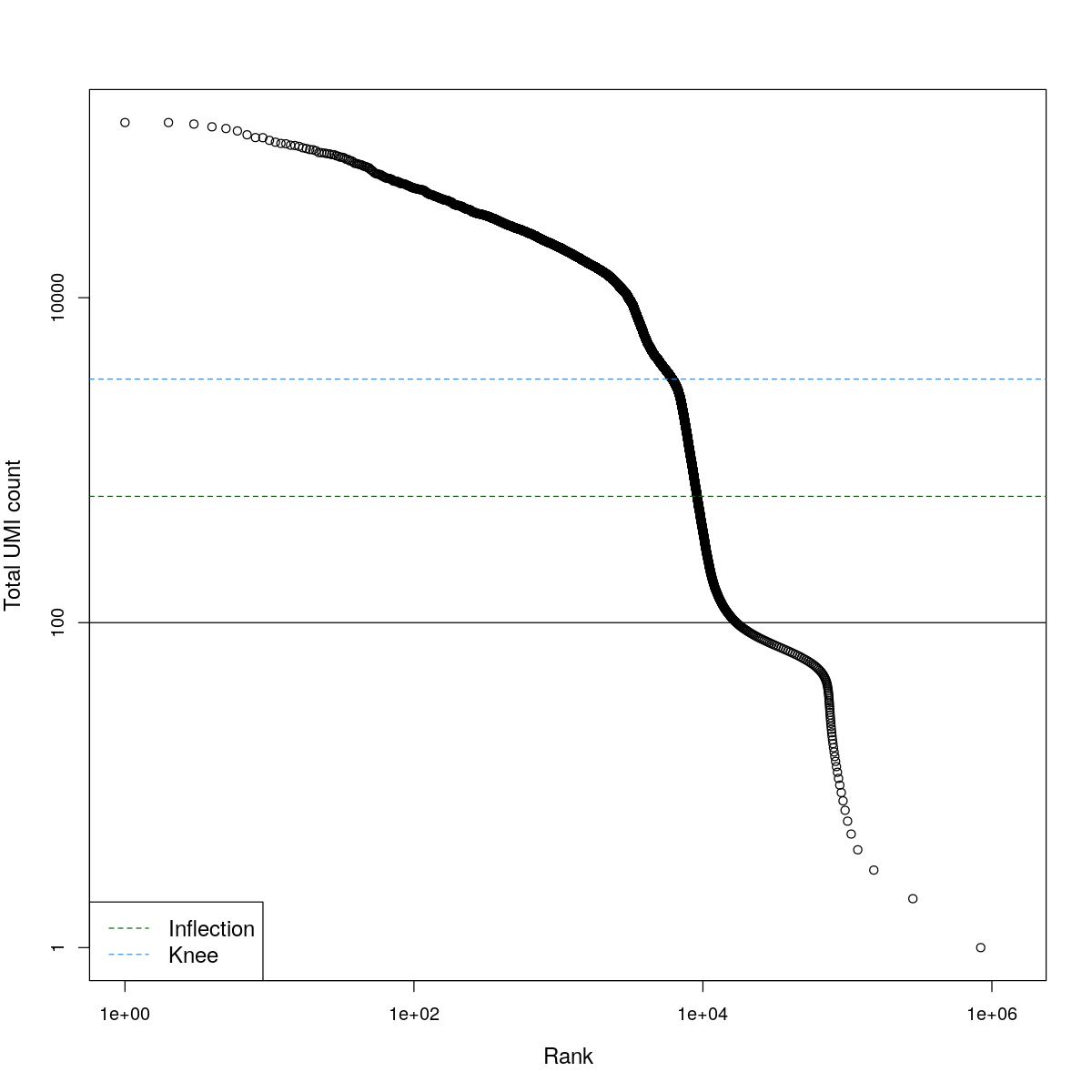
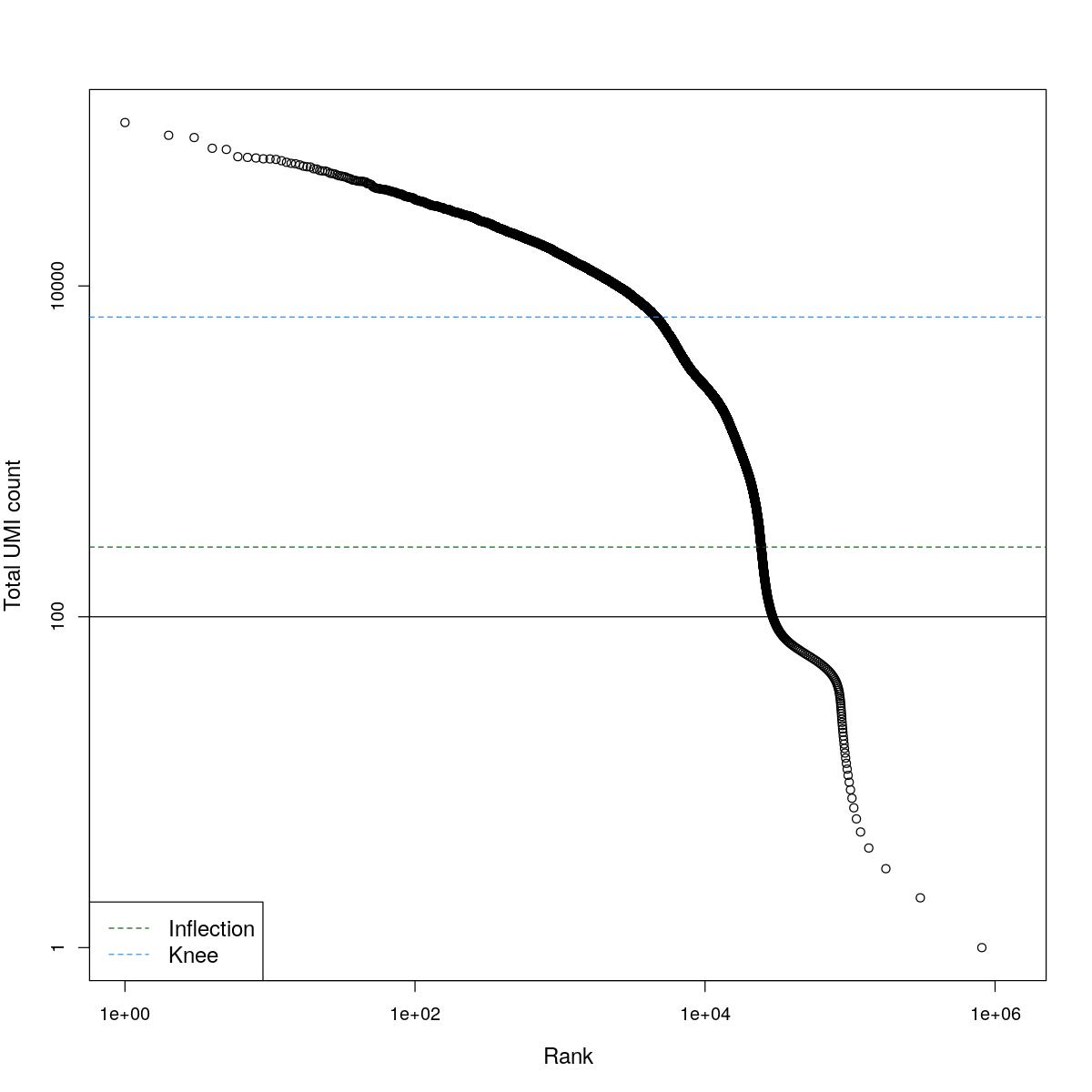
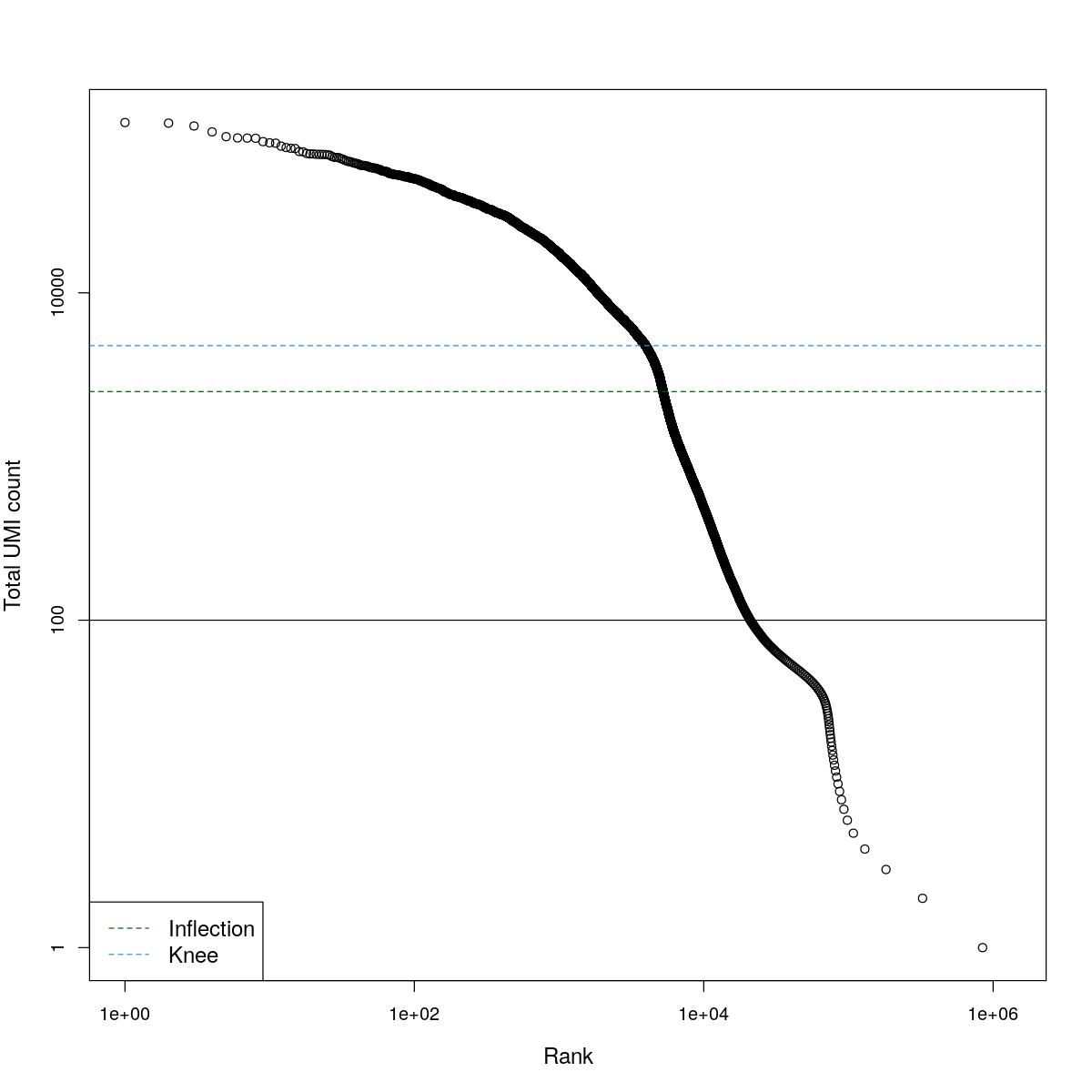
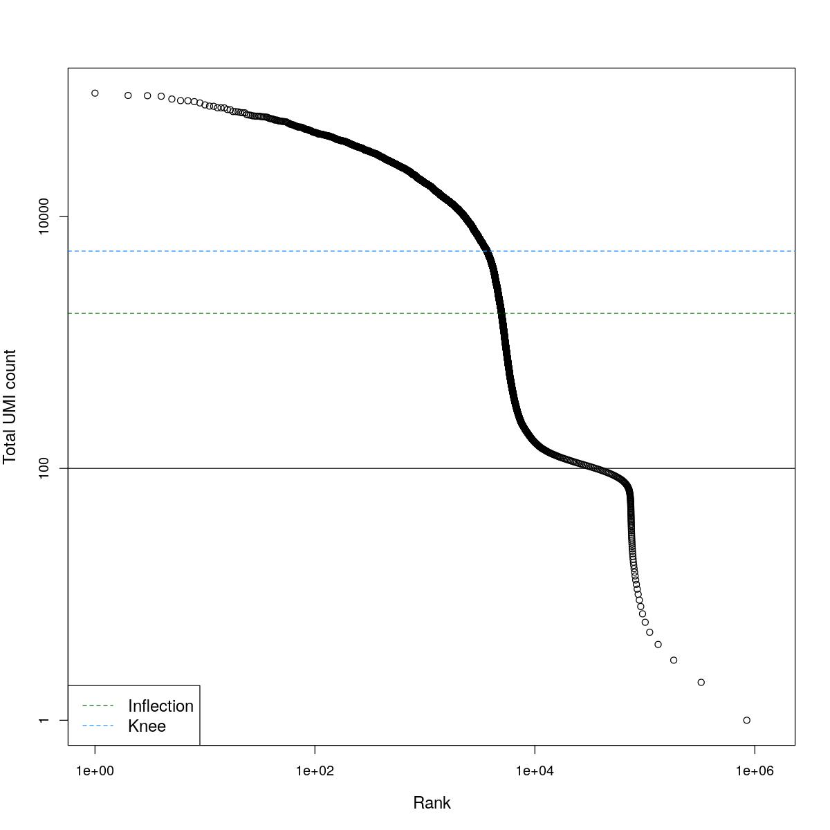
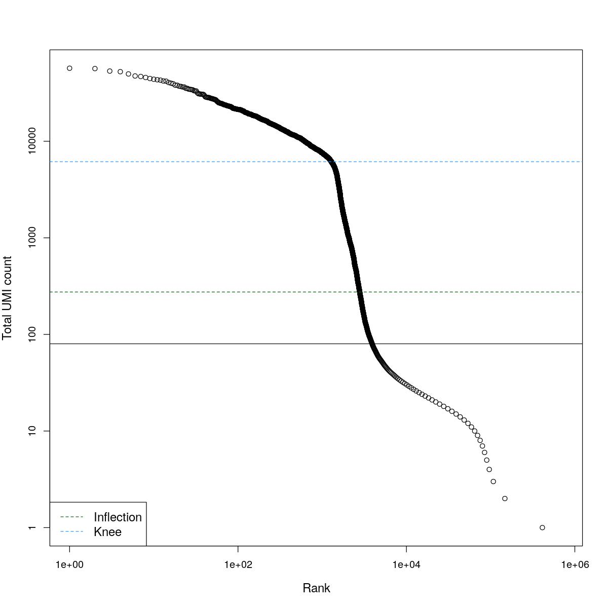
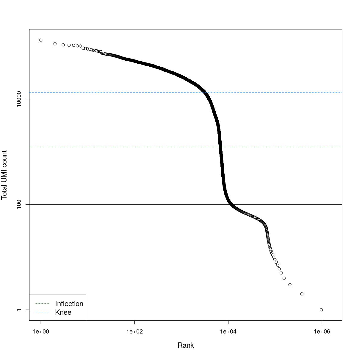
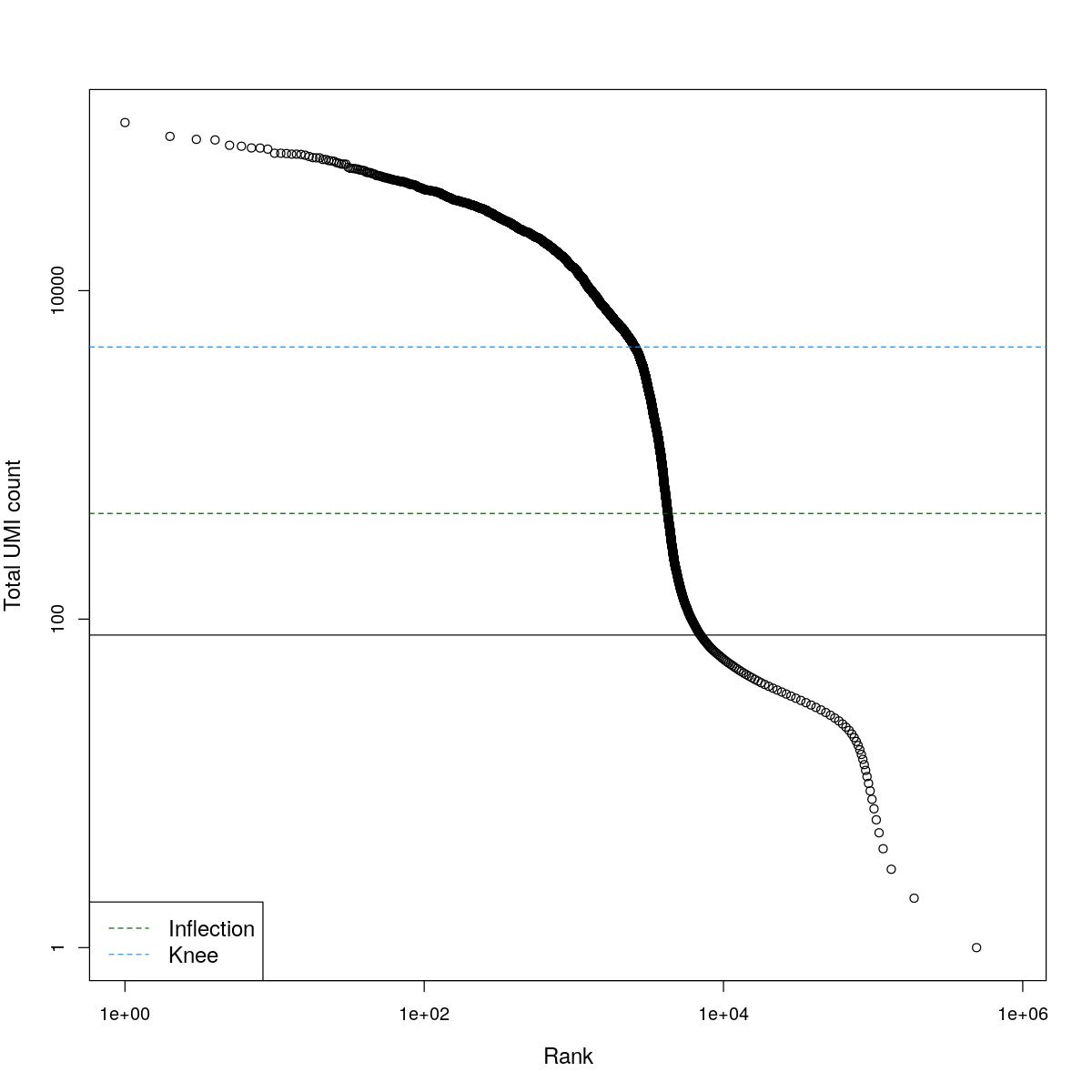
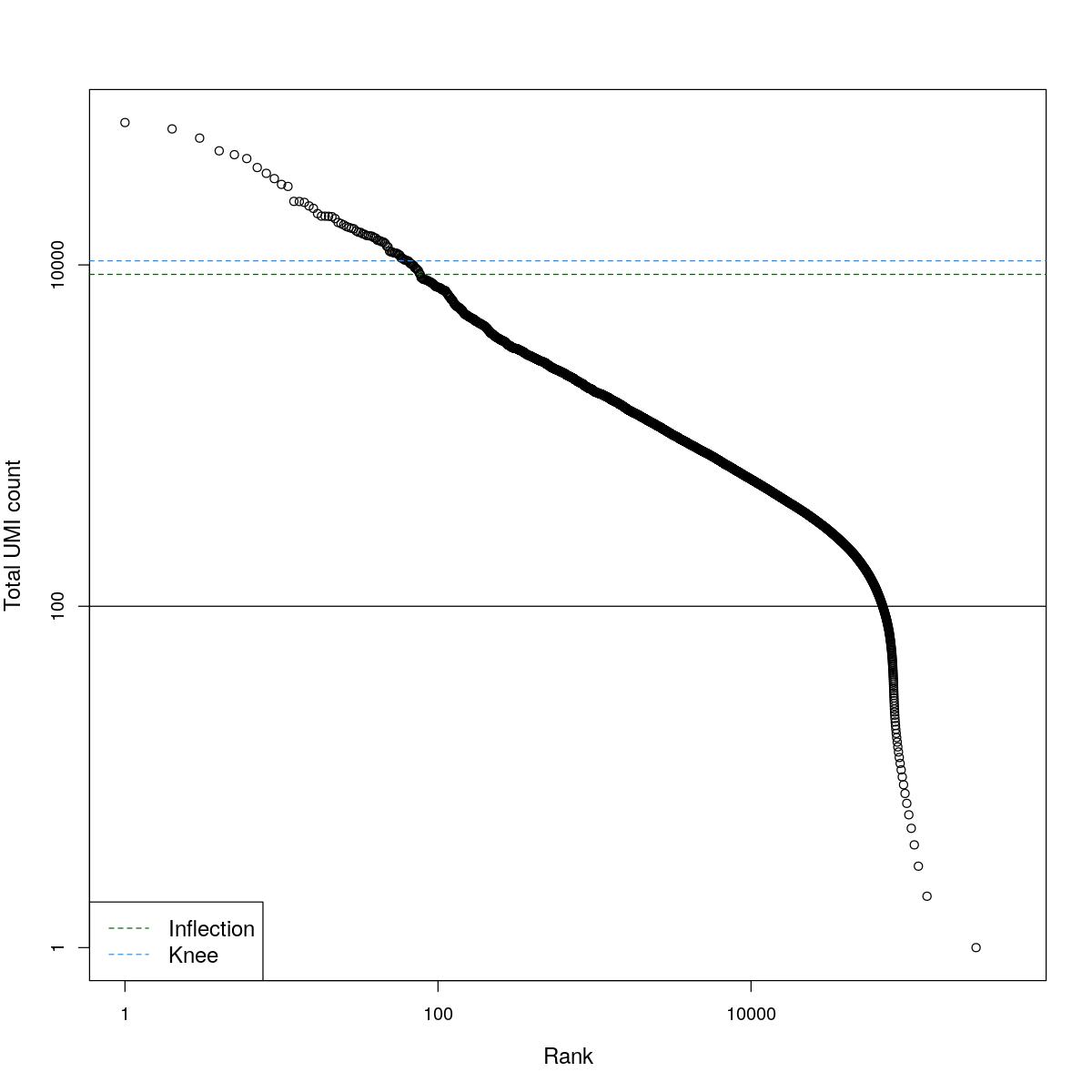
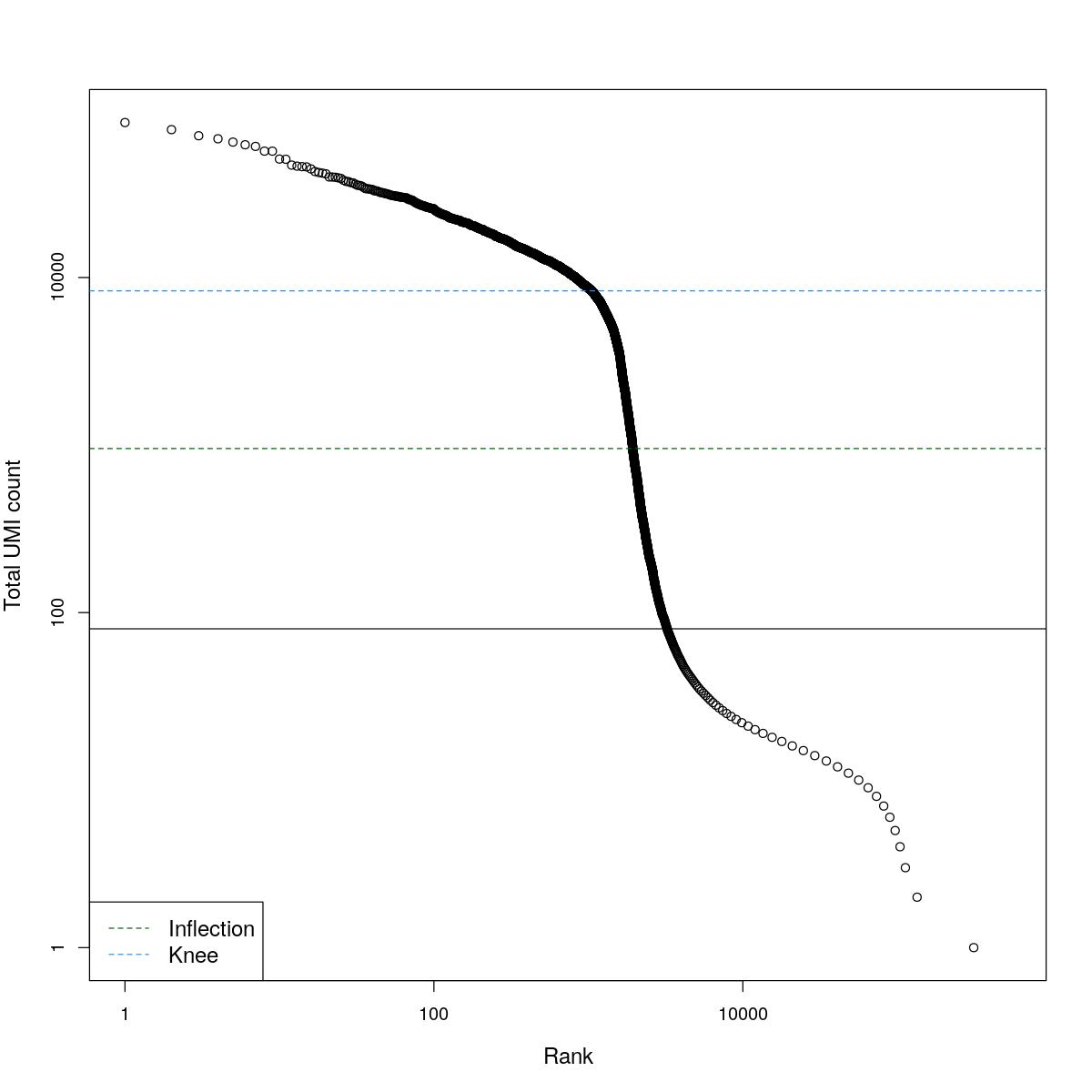
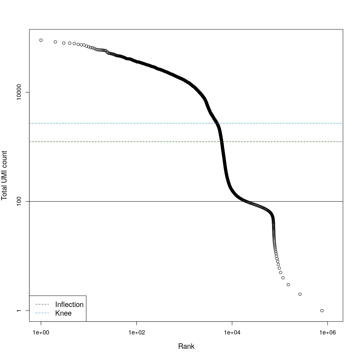
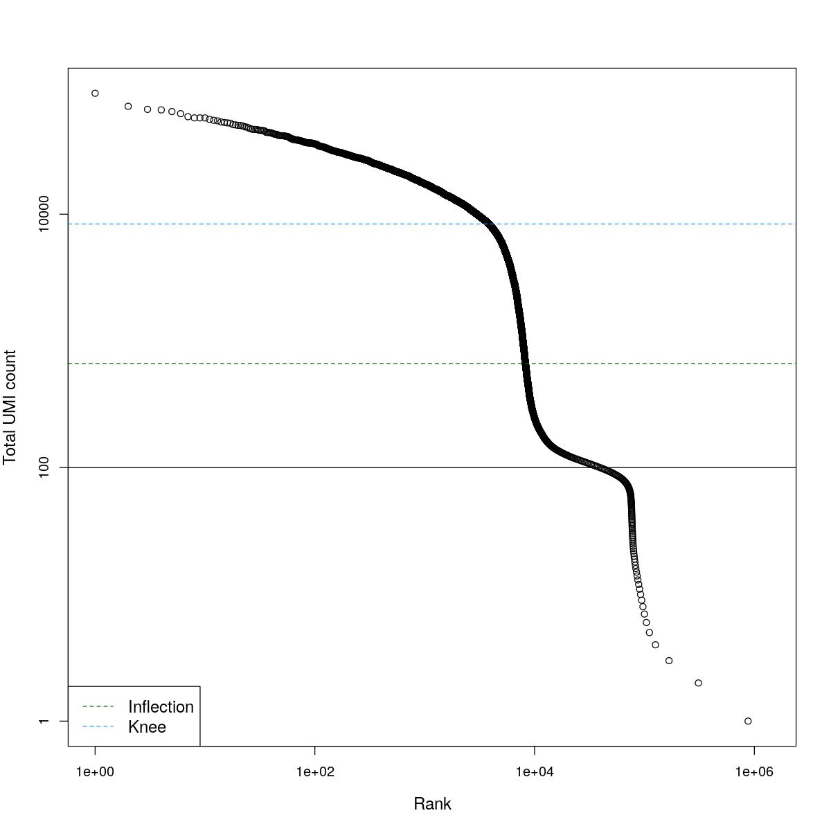
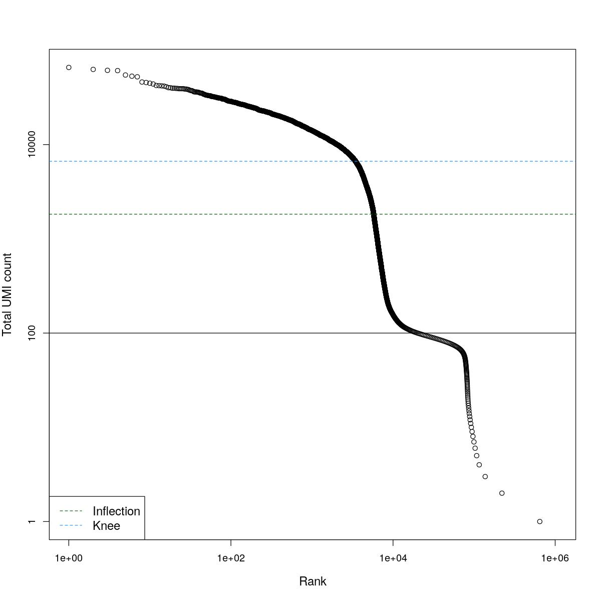
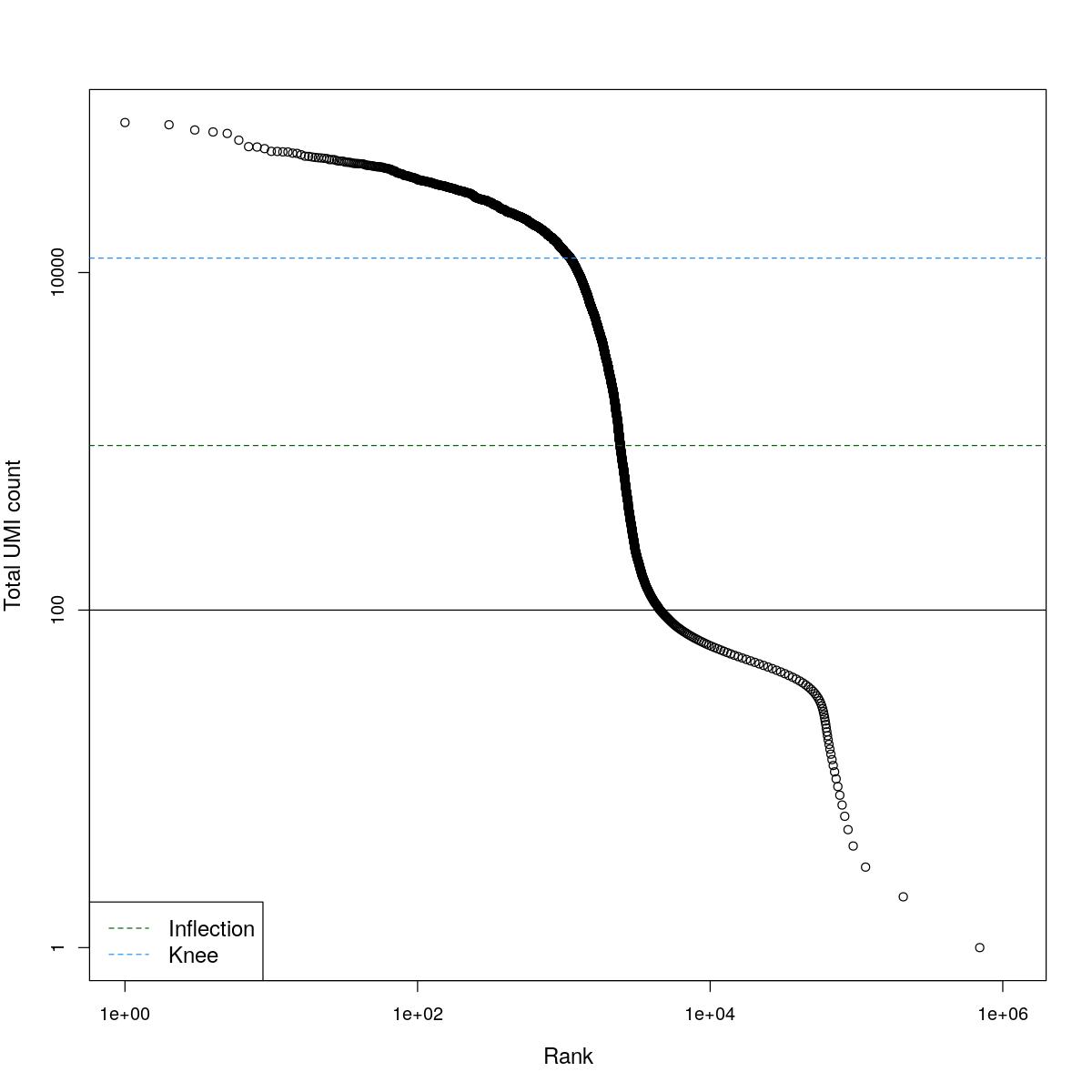
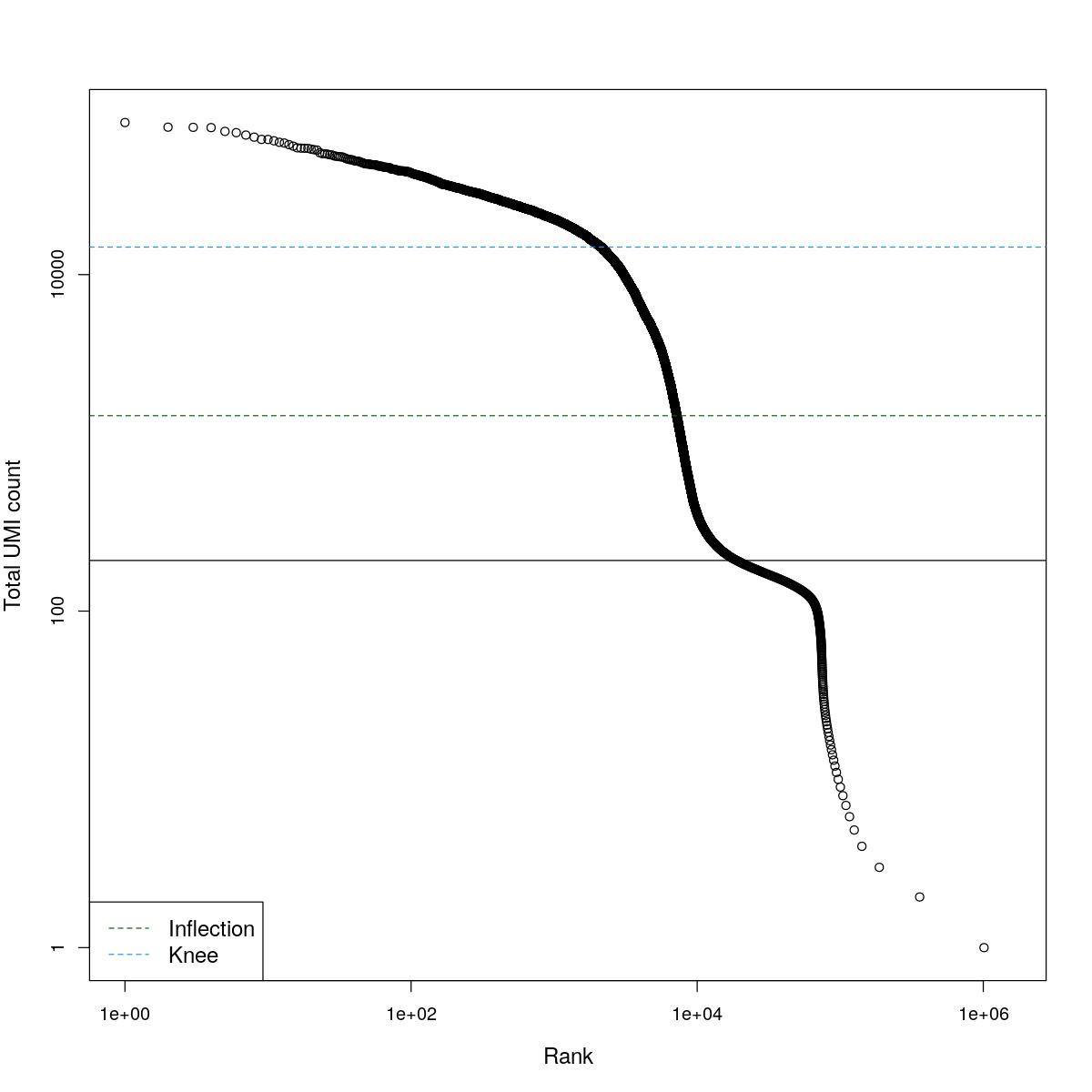
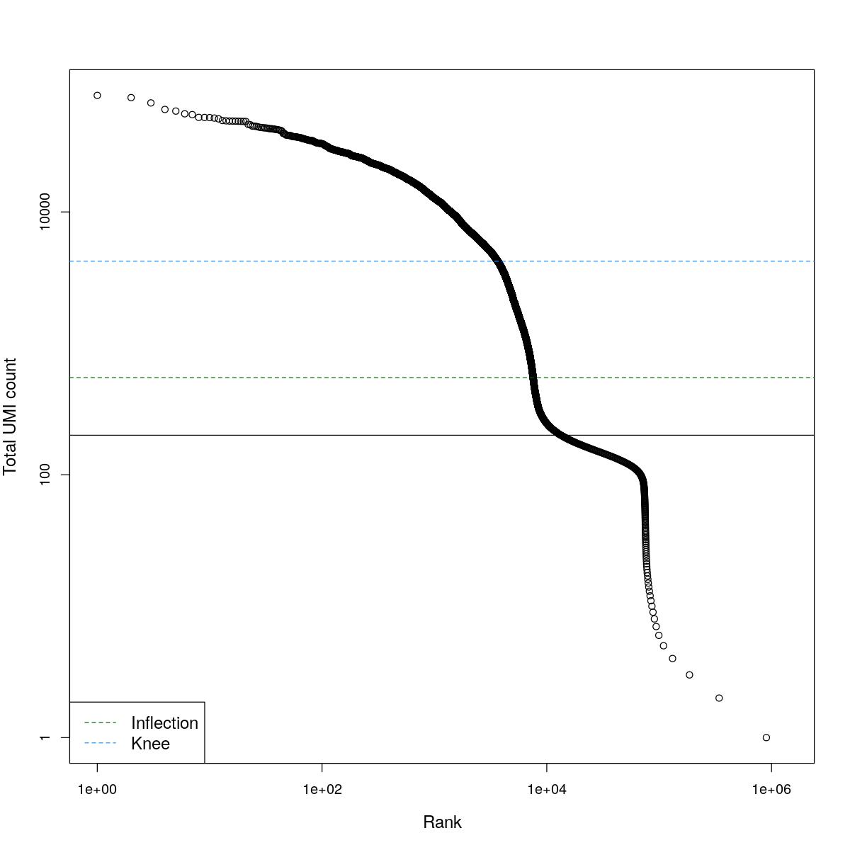
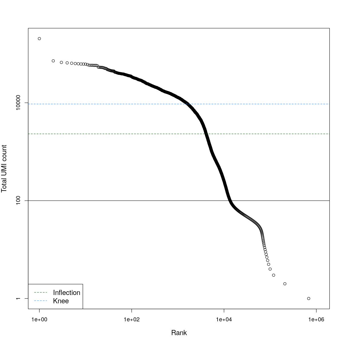
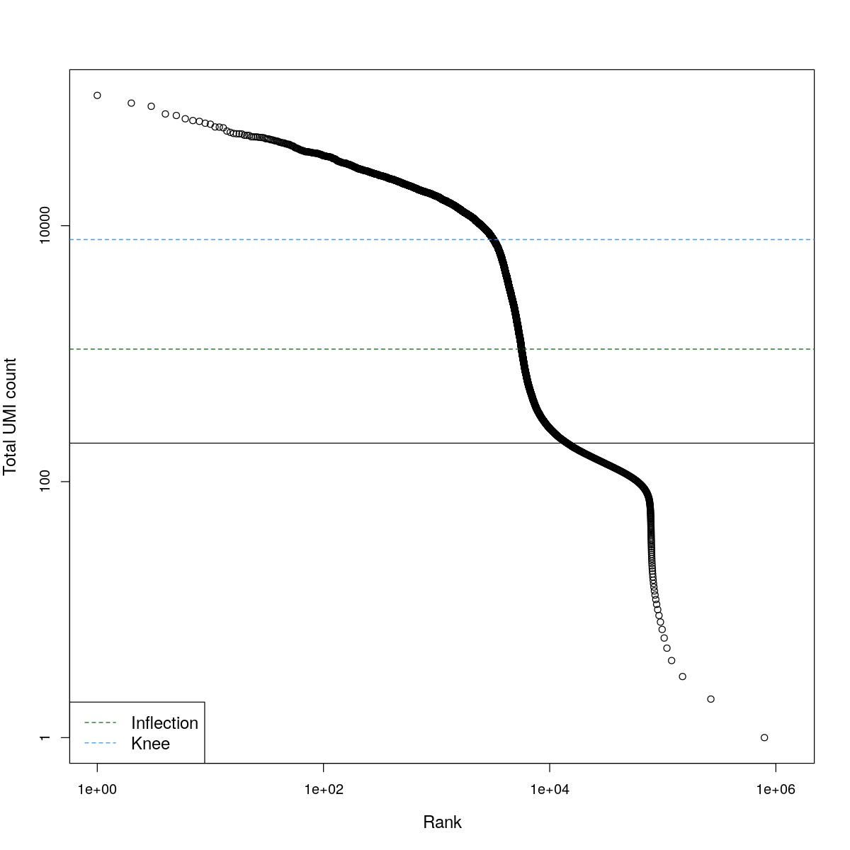
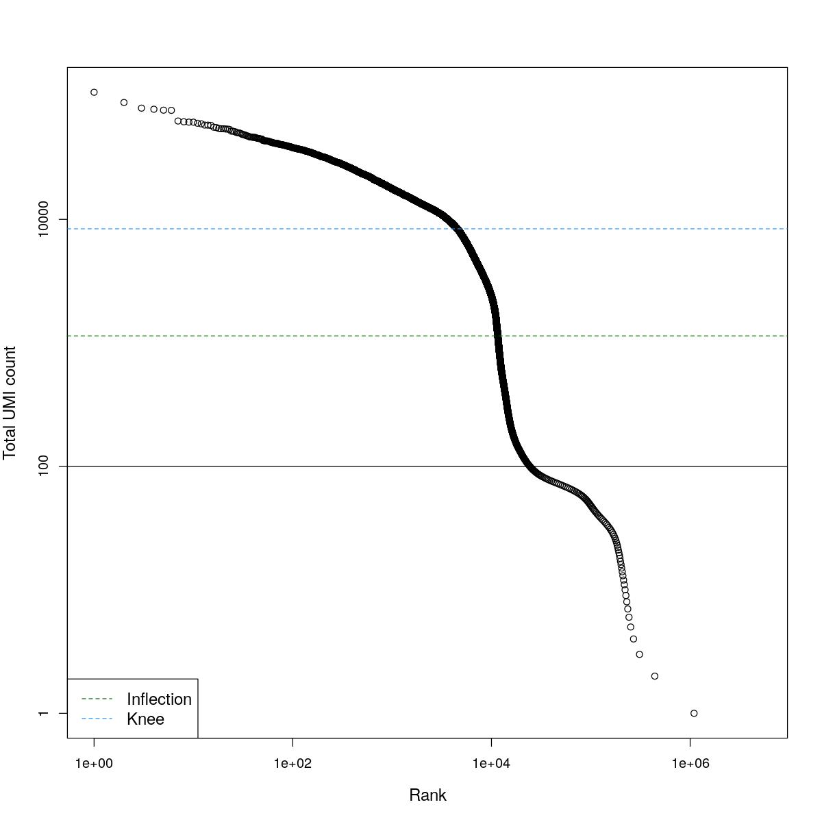
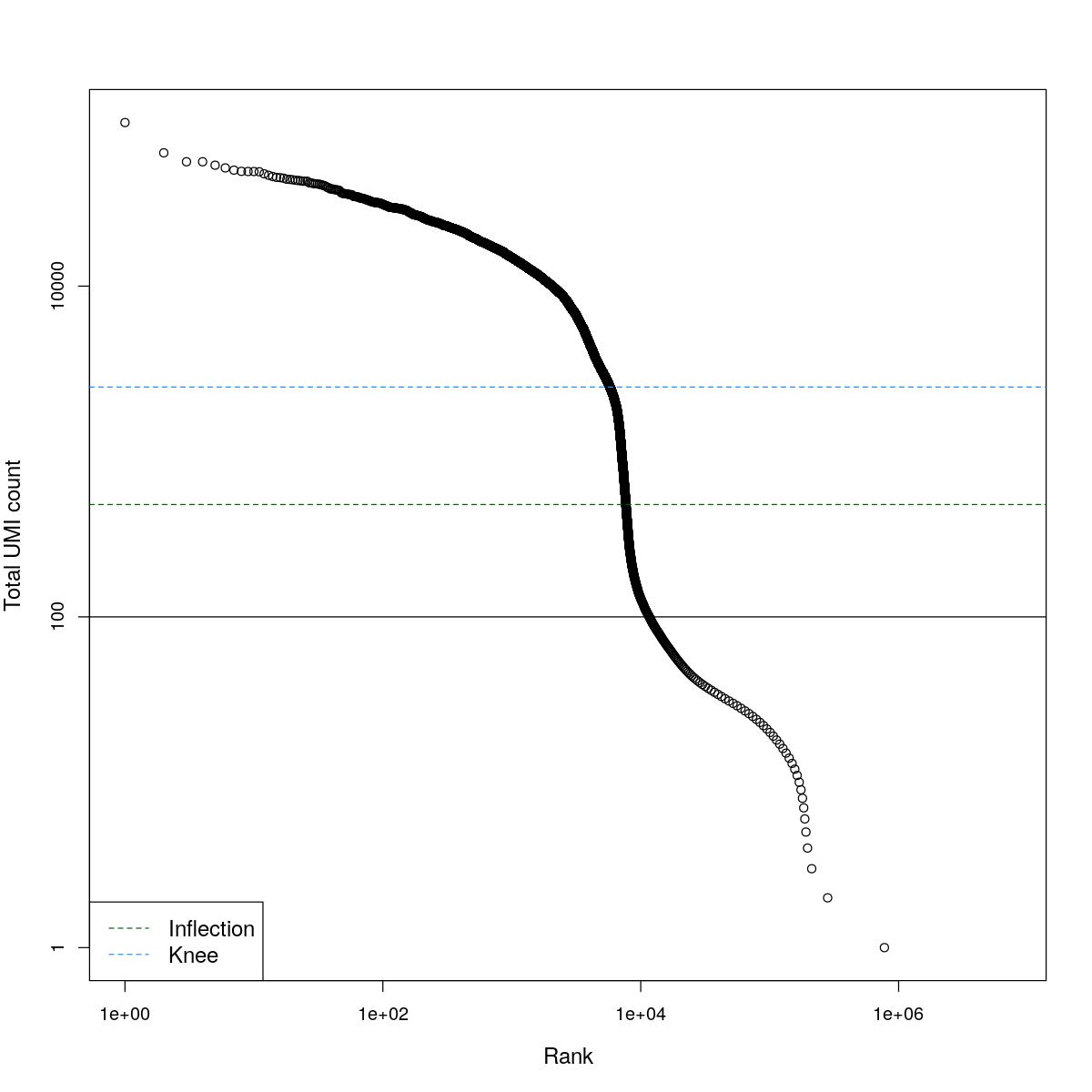
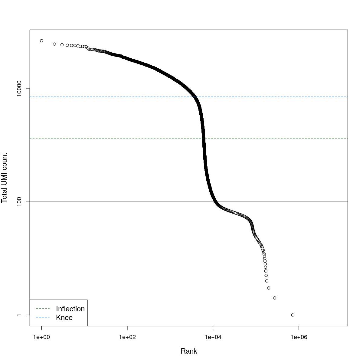
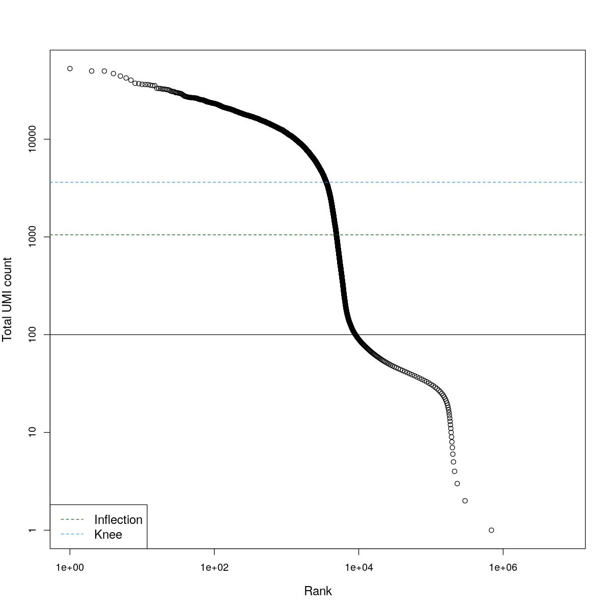
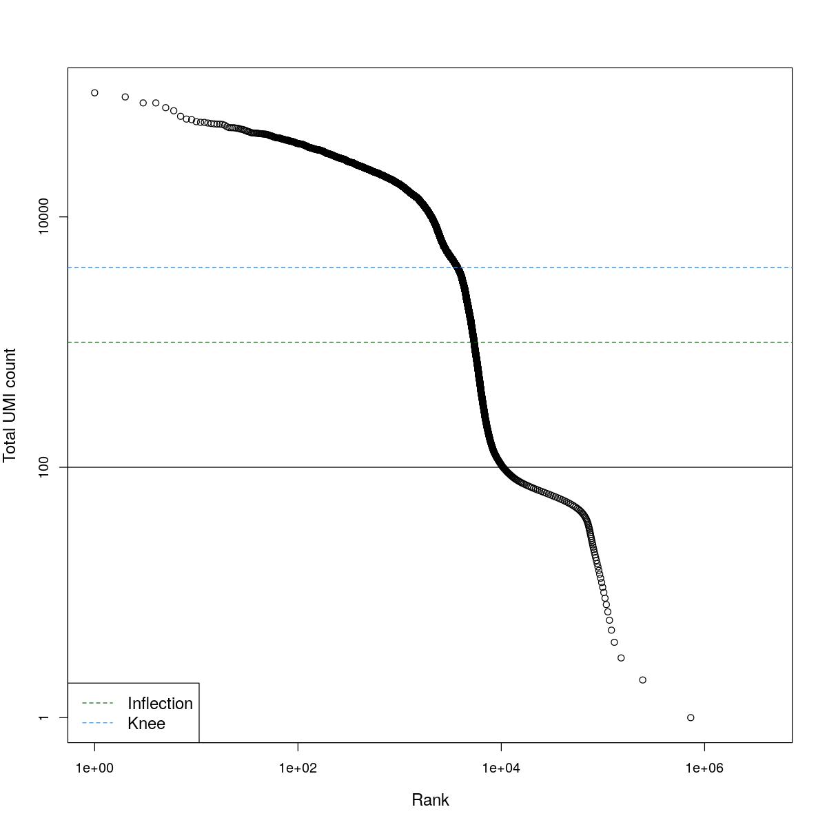
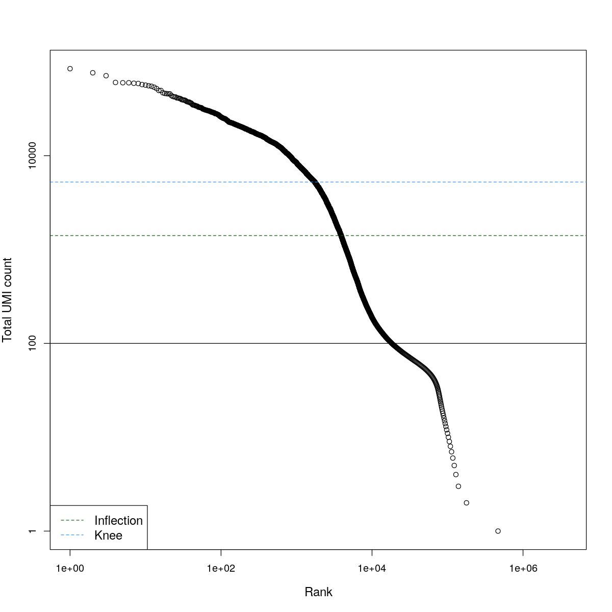
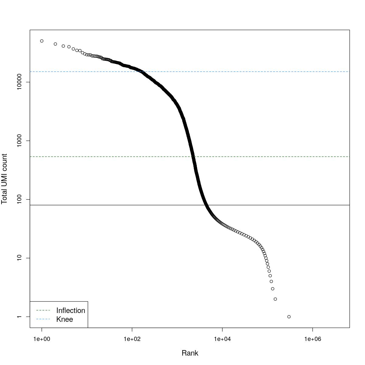
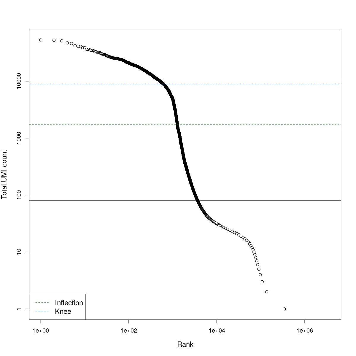
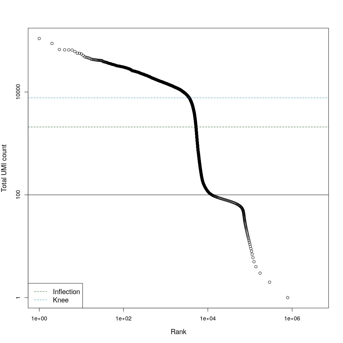
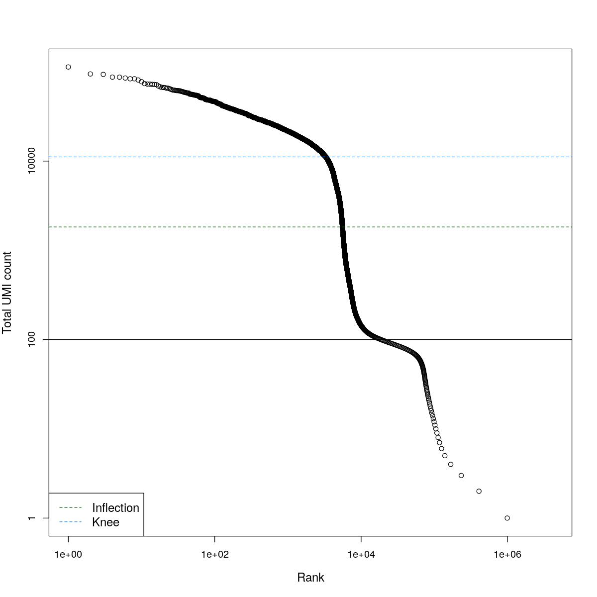
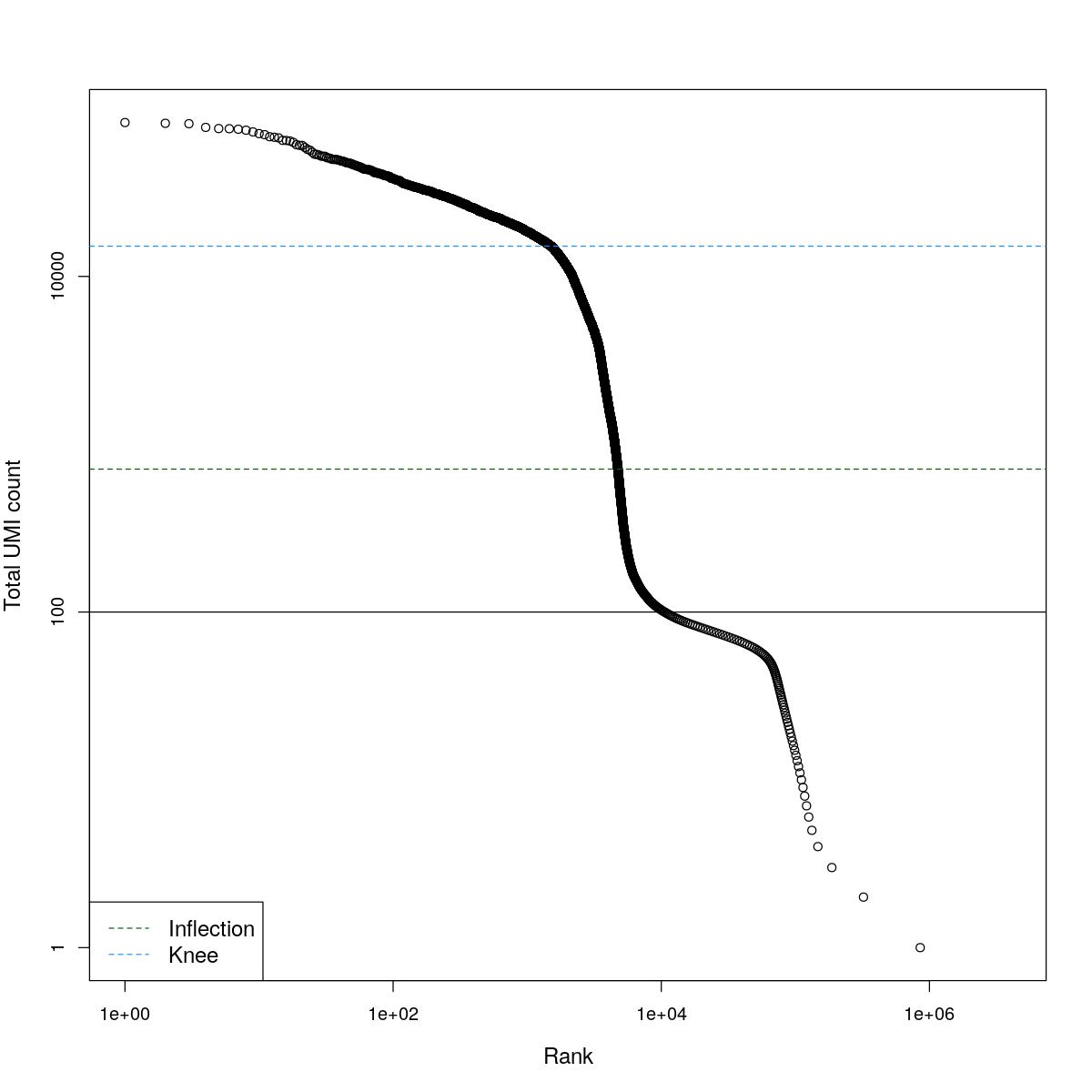
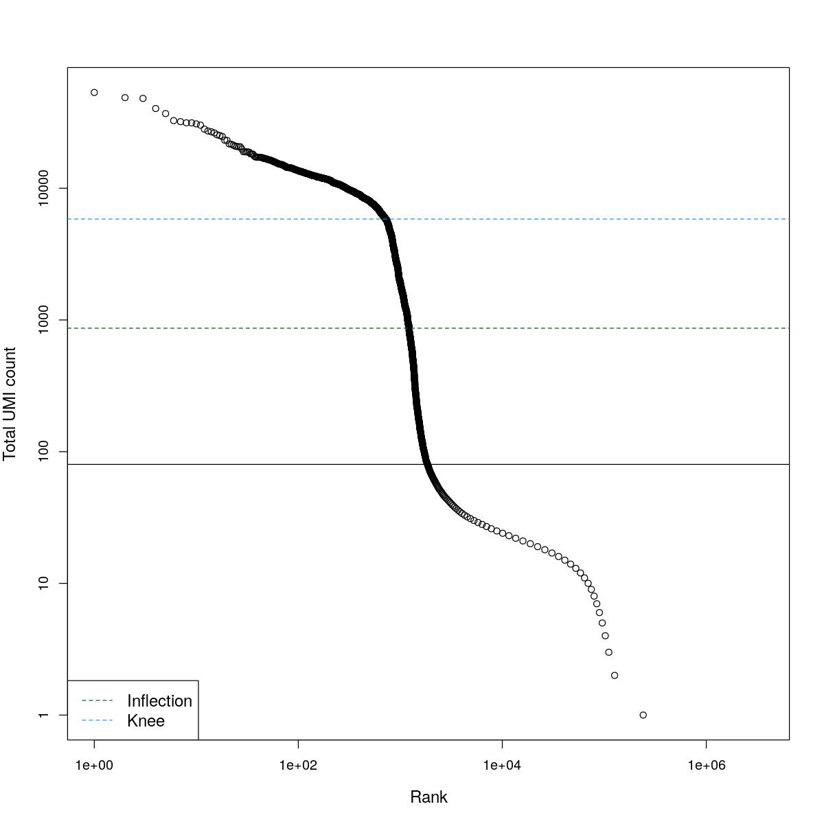
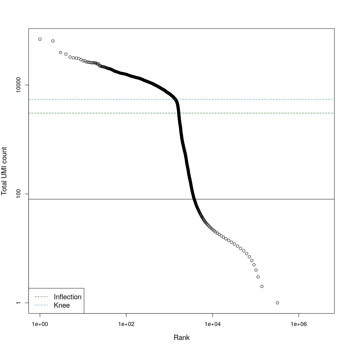
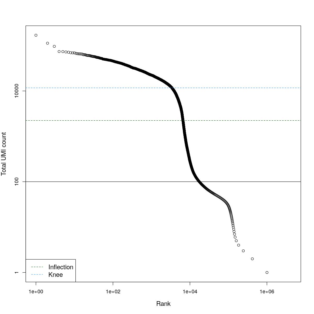
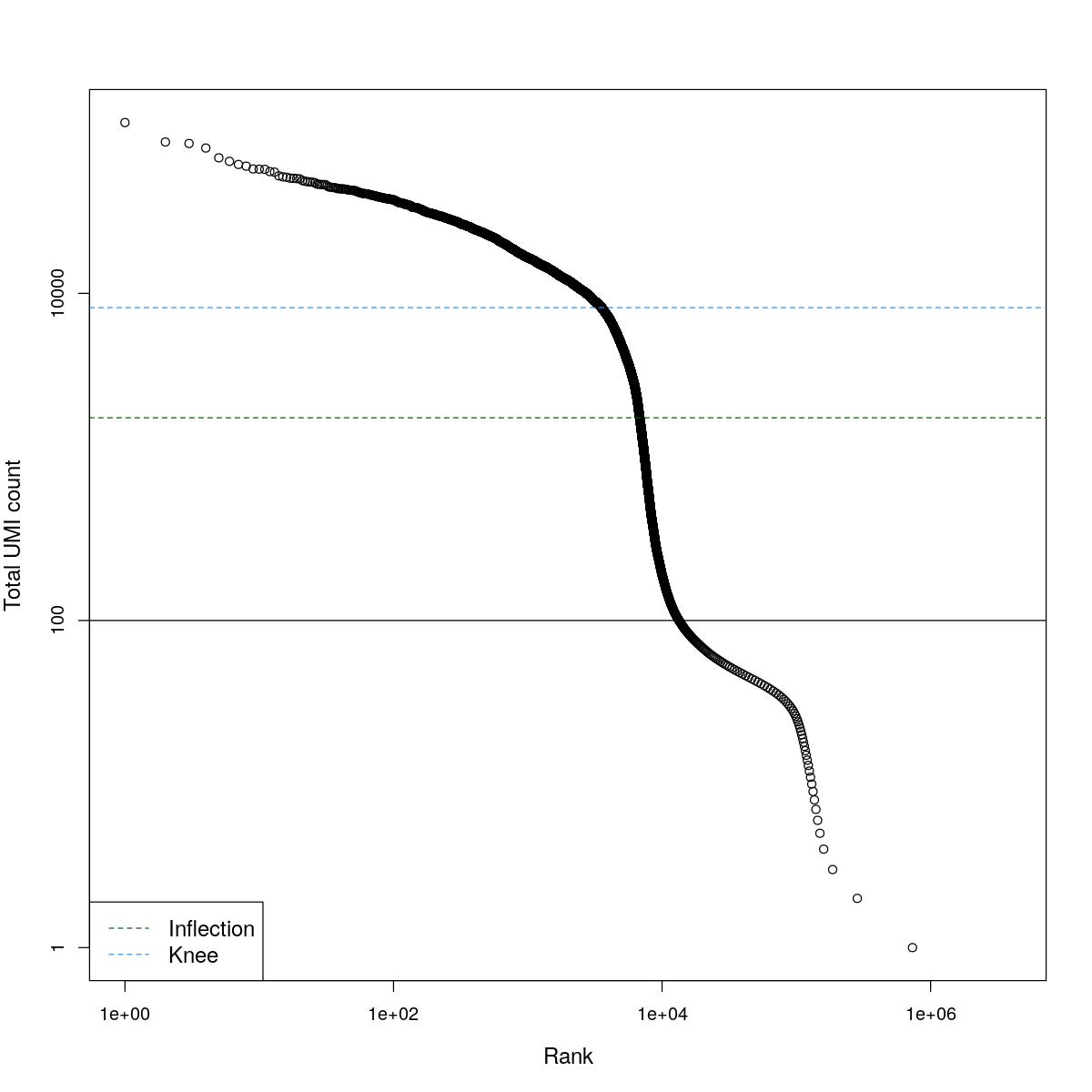
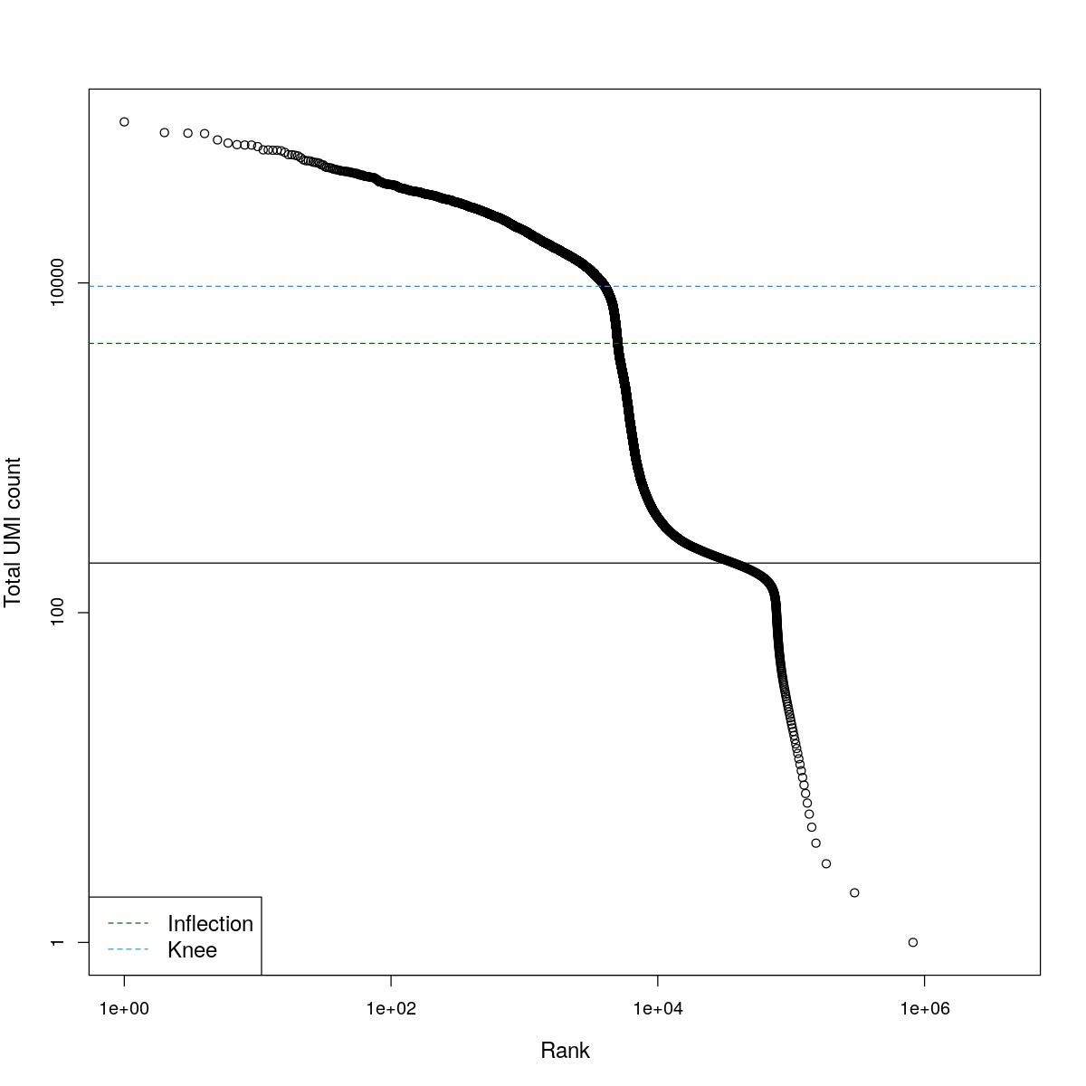
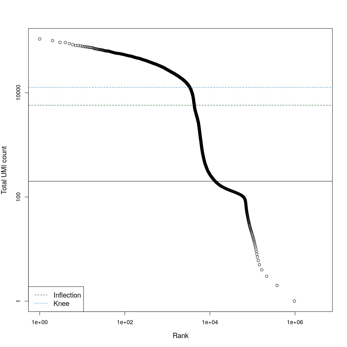
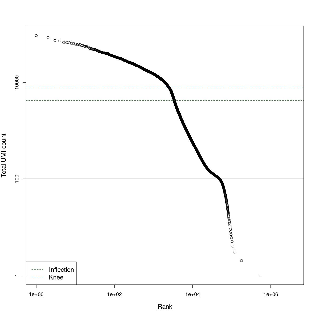
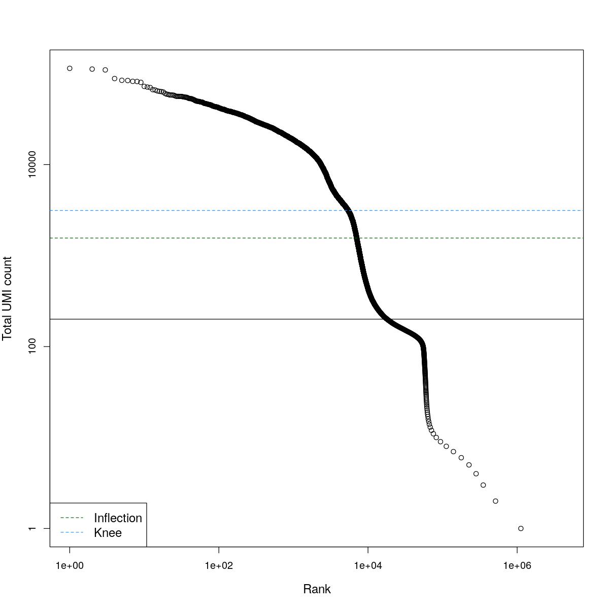
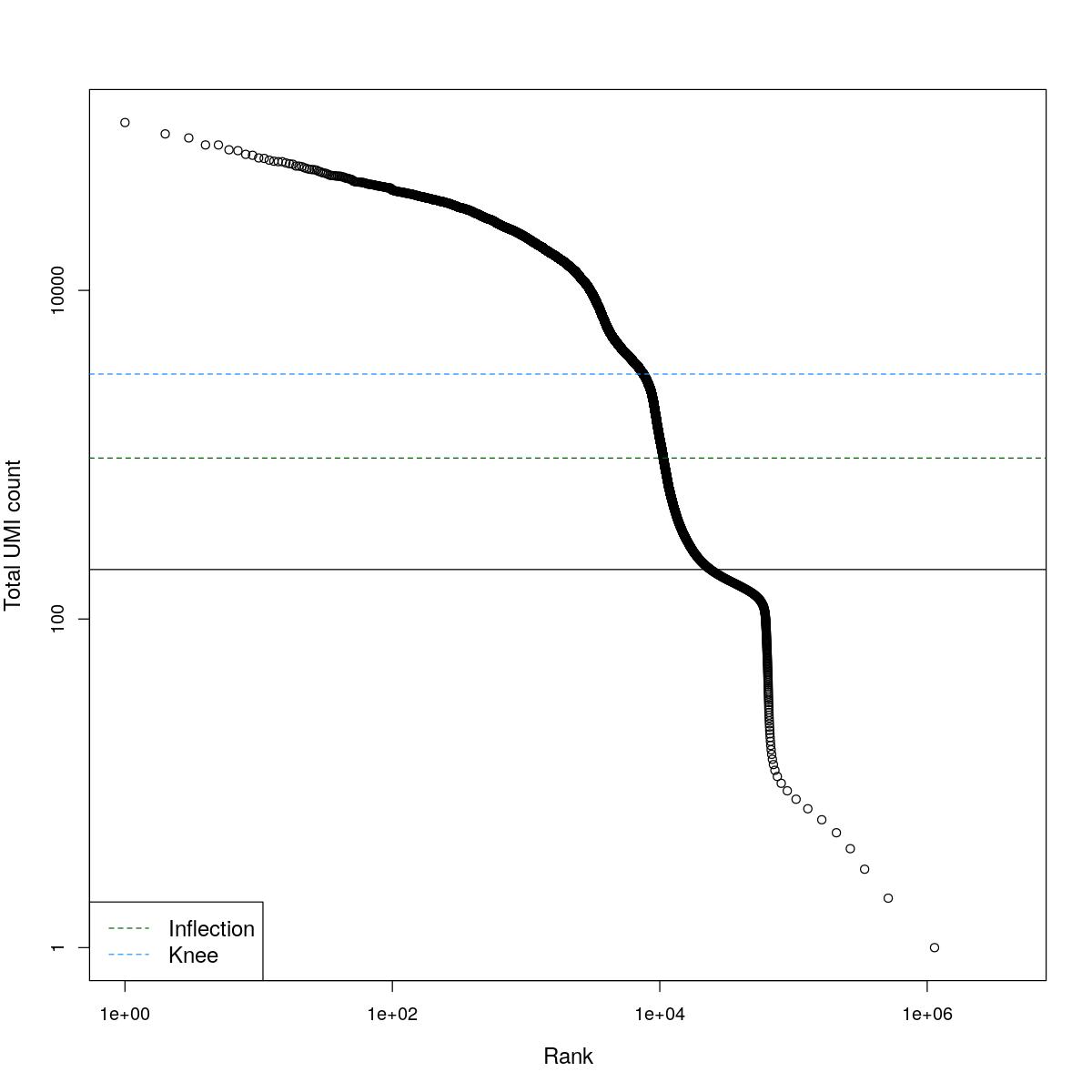
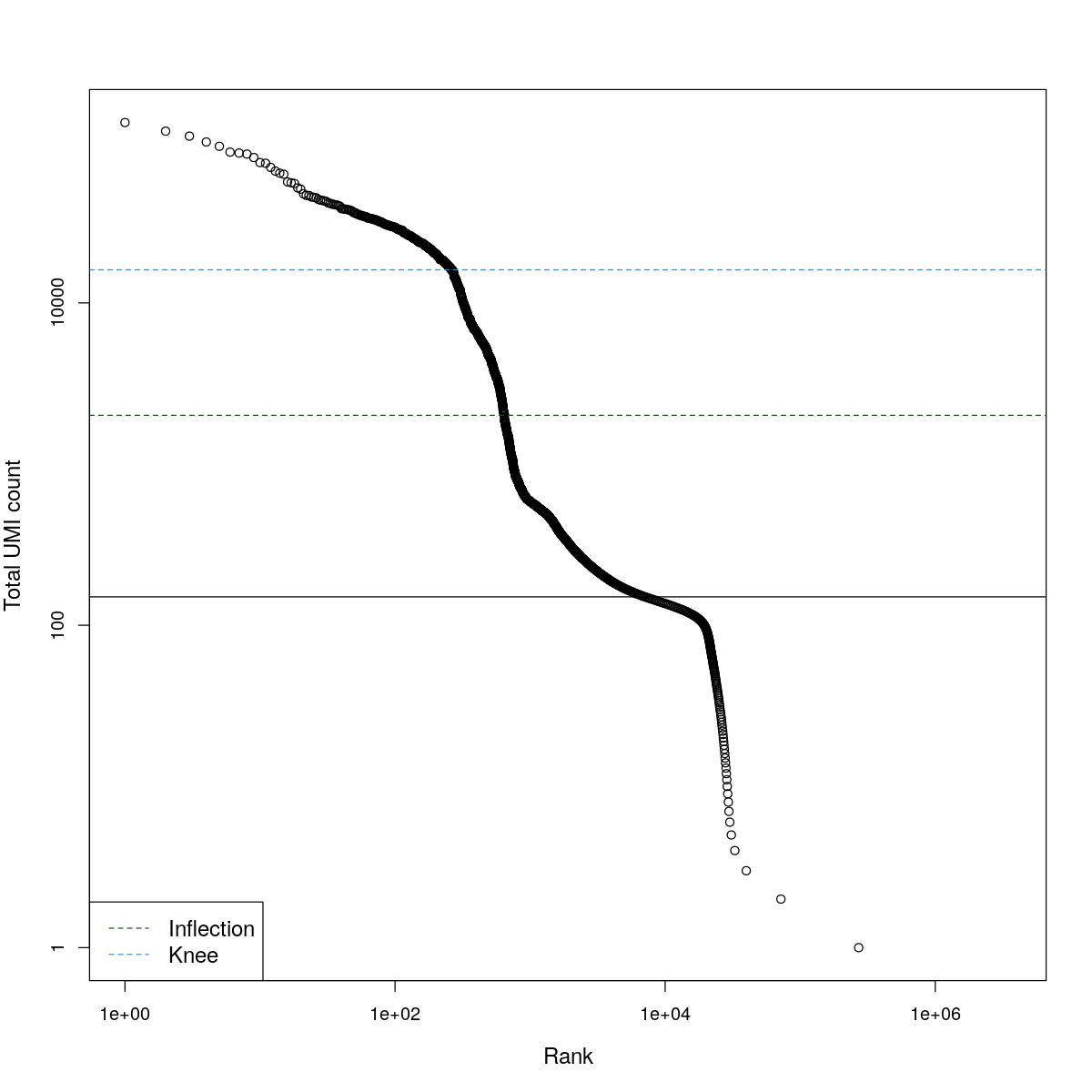
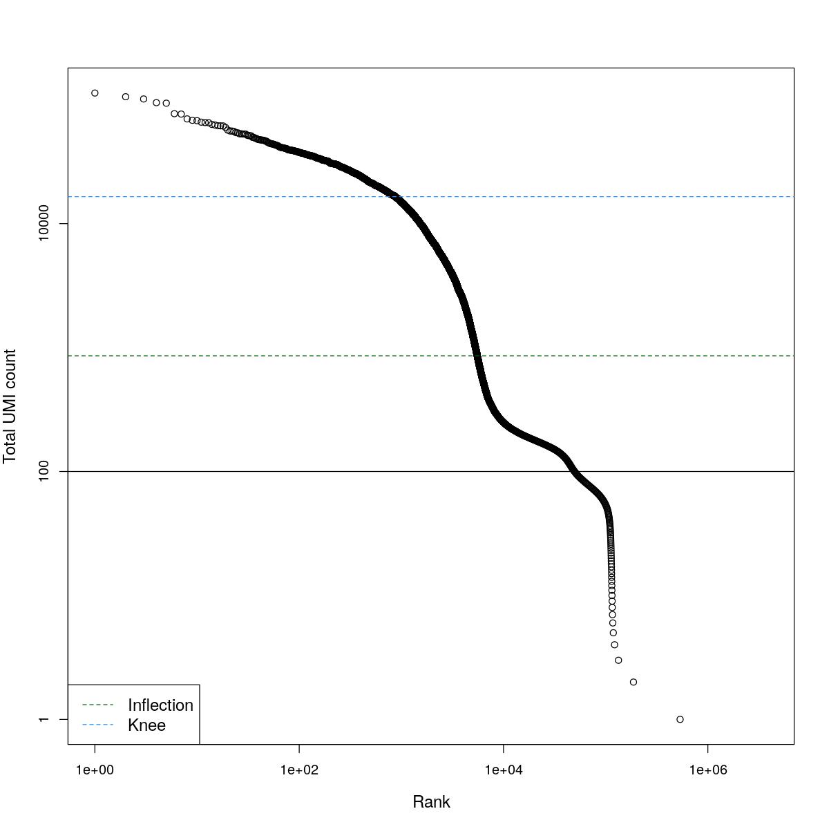
cat("### BCRank {.tabset}\n\n")BCRank
for(i in seq_along(res)){
  cat("#### ",names(res)[i],"\n\n")
  uniq <- !duplicated(res[[i]]$bcrank$rank)
  suppressWarnings(plot(res[[i]]$bcrank$rank[uniq], res[[i]]$bcrank$total[uniq], log="xy",
      xlab="Rank", ylab="Total UMI count", cex.lab=1.2))

  suppressWarnings(abline(h=metadata(res[[i]]$bcrank)$inflection, col="darkgreen", lty=2))
  suppressWarnings(abline(h=metadata(res[[i]]$bcrank)$knee, col="dodgerblue", lty=2))
  suppressWarnings(abline(h=res[[i]]$lower_cutoff))
  suppressWarnings(legend("bottomleft", legend=c("Inflection", "Knee"),
          col=c("darkgreen", "dodgerblue"), lty=2, cex=1.2))
  cat("\n\n")
}

for(i in seq_along(res)){
  print(names(res)[i])
  print(table(Sig=res[[i]]$e.out$FDR <= 0.001, Limited=res[[i]]$e.out$Limited))
  print(paste0(rep("-",80),collapse = ""))
}
[1] "o24300_1_01-79"
Limited
Sig FALSE TRUE
FALSE 1276866 0
TRUE 171 7777
[1] "--------------------------------------------------------------------------------"
[1] "o24300_1_02-86"
Limited
Sig FALSE TRUE
FALSE 1201081 0
TRUE 820 16081
[1] "--------------------------------------------------------------------------------"
[1] "o24300_1_03-83"
Limited
Sig FALSE TRUE
FALSE 1253493 0
TRUE 109 6040
[1] "--------------------------------------------------------------------------------"
[1] "o24300_1_04-84"
Limited
Sig FALSE TRUE
FALSE 1254880 0
TRUE 54 5090
[1] "--------------------------------------------------------------------------------"
[1] "o24300_1_05-78"
Limited
Sig FALSE TRUE
FALSE 641198 0
TRUE 3 2046
[1] "--------------------------------------------------------------------------------"
[1] "o24300_1_06-81"
Limited
Sig FALSE TRUE
FALSE 1430138 0
TRUE 37 6873
[1] "--------------------------------------------------------------------------------"
[1] "o24300_1_07-87"
Limited
Sig FALSE TRUE
FALSE 746471 0
TRUE 89 3538
[1] "--------------------------------------------------------------------------------"
[1] "o24300_1_11-80"
Limited
Sig FALSE TRUE
FALSE 387418 0
TRUE 6011 9865
[1] "--------------------------------------------------------------------------------"
[1] "o24300_1_12-89"
Limited
Sig FALSE TRUE
FALSE 471959 0
TRUE 1 1853
[1] "--------------------------------------------------------------------------------"
[1] "o24793_1_01-91"
Limited
Sig FALSE TRUE
FALSE 1163603 0
TRUE 715 4975
[1] "--------------------------------------------------------------------------------"
[1] "o24793_1_02-92"
Limited
Sig FALSE TRUE
FALSE 1325635 0
TRUE 41 6826
[1] "--------------------------------------------------------------------------------"
[1] "o24793_1_03-93"
Limited
Sig FALSE TRUE
FALSE 998455 0
TRUE 50 5839
[1] "--------------------------------------------------------------------------------"
[1] "o24793_1_04-95"
Limited
Sig FALSE TRUE
FALSE 1102702 0
TRUE 0 2320
[1] "--------------------------------------------------------------------------------"
[1] "o24793_1_05-96"
Limited
Sig FALSE TRUE
FALSE 1520866 0
TRUE 92 6546
[1] "--------------------------------------------------------------------------------"
[1] "o24793_1_06-98a"
Limited
Sig FALSE TRUE
FALSE 1336516 0
TRUE 592 3874
[1] "--------------------------------------------------------------------------------"
[1] "o24793_1_07-98b"
Limited
Sig FALSE TRUE
FALSE 1075768 0
TRUE 178 6613
[1] "--------------------------------------------------------------------------------"
[1] "o24793_1_08-99"
Limited
Sig FALSE TRUE
FALSE 1218827 0
TRUE 90 4958
[1] "--------------------------------------------------------------------------------"
[1] "26_comb"
Limited
Sig FALSE TRUE
FALSE 1633590 0
TRUE 138 11897
[1] "--------------------------------------------------------------------------------"
[1] "Aggr_23"
Limited
Sig FALSE TRUE
FALSE 1204295 0
TRUE 143 7158
[1] "--------------------------------------------------------------------------------"
[1] "Aggr_28"
Limited
Sig FALSE TRUE
FALSE 1102828 0
TRUE 87 5884
[1] "--------------------------------------------------------------------------------"
[1] "Aggr_31"
Limited
Sig FALSE TRUE
FALSE 1021960 0
TRUE 243 5368
[1] "--------------------------------------------------------------------------------"
[1] "o23841_1_01-53"
Limited
Sig FALSE TRUE
FALSE 1130506 0
TRUE 62 5123
[1] "--------------------------------------------------------------------------------"
[1] "o23841_1_02-54a"
Limited
Sig FALSE TRUE
FALSE 718656 0
TRUE 350 3416
[1] "--------------------------------------------------------------------------------"
[1] "o23841_1_03-54b"
Limited
Sig FALSE TRUE
FALSE 435097 0
TRUE 1 838
[1] "--------------------------------------------------------------------------------"
[1] "o23841_1_04-59"
Limited
Sig FALSE TRUE
FALSE 525357 0
TRUE 0 1562
[1] "--------------------------------------------------------------------------------"
[1] "o23841_1_05-62"
Limited
Sig FALSE TRUE
FALSE 1175186 0
TRUE 31 5506
[1] "--------------------------------------------------------------------------------"
[1] "o23841_1_06-64"
Limited
Sig FALSE TRUE
FALSE 1440747 0
TRUE 2 5702
[1] "--------------------------------------------------------------------------------"
[1] "o23841_1_07-74"
Limited
Sig FALSE TRUE
FALSE 1274442 0
TRUE 2 4666
[1] "--------------------------------------------------------------------------------"
[1] "o23841_1_08-75"
Limited
Sig FALSE TRUE
FALSE 343491 0
TRUE 0 1256
[1] "--------------------------------------------------------------------------------"
[1] "o23841_1_10-76"
Limited
Sig FALSE TRUE
FALSE 478076 0
TRUE 20 2725
[1] "--------------------------------------------------------------------------------"
[1] "o23841_1_11-077W"
Limited
Sig FALSE TRUE
FALSE 1449723 0
TRUE 106 7800
[1] "--------------------------------------------------------------------------------"
[1] "o23841_1_12-077K"
Limited
Sig FALSE TRUE
FALSE 1095398 0
TRUE 156 7435
[1] "--------------------------------------------------------------------------------"
[1] "o23841_1_14-72DMSO"
Limited
Sig FALSE TRUE
FALSE 1242348 0
TRUE 40 5677
[1] "--------------------------------------------------------------------------------"
[1] "o23841_1_15-72Tofa"
Limited
Sig FALSE TRUE
FALSE 1428447 0
TRUE 78 5753
[1] "--------------------------------------------------------------------------------"
[1] "o24555_1_1-94_tofa"
Limited
Sig FALSE TRUE
FALSE 1232194 0
TRUE 200 8326
[1] "--------------------------------------------------------------------------------"
[1] "o24555_1_2-94_control1"
Limited
Sig FALSE TRUE
FALSE 828522 0
TRUE 673 6831
[1] "--------------------------------------------------------------------------------"
[1] "SynBio_Tofacitinib"
Limited
Sig FALSE TRUE
FALSE 1601179 0
TRUE 796 7323
[1] "--------------------------------------------------------------------------------"
[1] "SynBio_Untreated"
Limited
Sig FALSE TRUE
FALSE 1620526 0
TRUE 612 10046
[1] "--------------------------------------------------------------------------------"
[1] "SynTissue_49_8000"
Limited
Sig FALSE TRUE
FALSE 442527 0
TRUE 1 943
[1] "--------------------------------------------------------------------------------"
[1] "SynTissue_50_6000"
Limited
Sig FALSE TRUE
FALSE 833419 0
TRUE 99 4514
[1] "--------------------------------------------------------------------------------"cat("### Pval hist {.tabset}\n\n")Pval hist
for(i in seq_along(res)){
  cat("#### ",names(res)[i],"\n\n")
  print(hist(res[[i]]$e.out$PValue[res[[i]]$e.out$Total <= res[[i]]$lower_cutoff & res[[i]]$e.out$Total > 0],
    xlab="P-value", main="", col="grey80"))
  cat("\n\n")
}
o24300_1_01-79
![]()
$breaks [1] 0.00 0.05 0.10 0.15 0.20 0.25 0.30 0.35 0.40 0.45 0.50 0.55 0.60 0.65 0.70 [16] 0.75 0.80 0.85 0.90 0.95 1.00
$counts [1] 62622 57311 55036 56043 55863 56599 57540 57530 58940 55861 62751 62482 [13] 60989 65441 63369 67097 80772 69945 78613 83056
$density [1] 0.9878378 0.9040588 0.8681716 0.8840566 0.8812172 0.8928273 0.9076712 [8] 0.9075134 0.9297557 0.8811856 0.9898727 0.9856293 0.9620778 1.0323064 [15] 0.9996214 1.0584292 1.2741470 1.1033553 1.2400896 1.3101762
$mids [1] 0.025 0.075 0.125 0.175 0.225 0.275 0.325 0.375 0.425 0.475 0.525 0.575 [13] 0.625 0.675 0.725 0.775 0.825 0.875 0.925 0.975
\(xname [1] "res[[i]]\)e.out\(PValue[res[[i]]\)e.out\(Total <= res[[i]]\)lower_cutoff & res[[i]]\(e.out\)Total > 0]"
$equidist [1] TRUE
attr(,“class”) [1] “histogram”
o24300_1_02-86
![]()
$breaks [1] 0.00 0.05 0.10 0.15 0.20 0.25 0.30 0.35 0.40 0.45 0.50 0.55 0.60 0.65 0.70 [16] 0.75 0.80 0.85 0.90 0.95 1.00
$counts [1] 66030 61157 58528 59128 57733 57186 56867 56725 55922 54721 56621 56415 [13] 55467 54317 57184 57047 62624 73031 78794 53267
$density [1] 1.1109017 1.0289174 0.9846866 0.9947811 0.9713114 0.9621085 0.9567416 [8] 0.9543526 0.9408428 0.9206369 0.9526029 0.9491371 0.9331877 0.9138399 [15] 0.9620749 0.9597700 1.0535985 1.2286879 1.3256458 0.8961745
$mids [1] 0.025 0.075 0.125 0.175 0.225 0.275 0.325 0.375 0.425 0.475 0.525 0.575 [13] 0.625 0.675 0.725 0.775 0.825 0.875 0.925 0.975
\(xname [1] "res[[i]]\)e.out\(PValue[res[[i]]\)e.out\(Total <= res[[i]]\)lower_cutoff & res[[i]]\(e.out\)Total > 0]"
$equidist [1] TRUE
attr(,“class”) [1] “histogram”
o24300_1_03-83
![]()
$breaks [1] 0.00 0.05 0.10 0.15 0.20 0.25 0.30 0.35 0.40 0.45 0.50 0.55 0.60 0.65 0.70 [16] 0.75 0.80 0.85 0.90 0.95 1.00
$counts [1] 70333 59838 58867 57464 59098 59362 58791 58000 60110 62832 [11] 67017 61881 69926 66594 52759 67235 105865 63263 56819 22696
$density [1] 1.1355479 0.9661029 0.9504258 0.9277740 0.9541554 0.9584178 0.9491988 [8] 0.9364279 0.9704945 1.0144420 1.0820101 0.9990878 1.1289768 1.0751806 [15] 0.8518103 1.0855298 1.7092230 1.0214006 0.9173602 0.3664339
$mids [1] 0.025 0.075 0.125 0.175 0.225 0.275 0.325 0.375 0.425 0.475 0.525 0.575 [13] 0.625 0.675 0.725 0.775 0.825 0.875 0.925 0.975
\(xname [1] "res[[i]]\)e.out\(PValue[res[[i]]\)e.out\(Total <= res[[i]]\)lower_cutoff & res[[i]]\(e.out\)Total > 0]"
$equidist [1] TRUE
attr(,“class”) [1] “histogram”
o24300_1_04-84
![]()
$breaks [1] 0.00 0.05 0.10 0.15 0.20 0.25 0.30 0.35 0.40 0.45 0.50 0.55 0.60 0.65 0.70 [16] 0.75 0.80 0.85 0.90 0.95 1.00
$counts [1] 60102 53641 53336 53177 51986 52884 52072 52439 53325 52772 53905 55511 [13] 60404 61030 60958 66769 72486 85530 93688 79040
$density [1] 0.9812131 0.8757321 0.8707527 0.8681569 0.8487129 0.8633735 0.8501169 [8] 0.8561085 0.8705732 0.8615450 0.8800421 0.9062614 0.9861435 0.9963634 [15] 0.9951880 1.0900572 1.1833918 1.3963455 1.5295313 1.2903910
$mids [1] 0.025 0.075 0.125 0.175 0.225 0.275 0.325 0.375 0.425 0.475 0.525 0.575 [13] 0.625 0.675 0.725 0.775 0.825 0.875 0.925 0.975
\(xname [1] "res[[i]]\)e.out\(PValue[res[[i]]\)e.out\(Total <= res[[i]]\)lower_cutoff & res[[i]]\(e.out\)Total > 0]"
$equidist [1] TRUE
attr(,“class”) [1] “histogram”
o24300_1_05-78
![]()
$breaks [1] 0.00 0.05 0.10 0.15 0.20 0.25 0.30 0.35 0.40 0.45 0.50 0.55 0.60 0.65 0.70 [16] 0.75 0.80 0.85 0.90 0.95 1.00
$counts [1] 37670 30818 29554 29450 28812 28883 29513 29980 29459 28920 29322 31664 [13] 33835 35581 34898 32972 33856 36503 34719 32926
$density [1] 1.1784119 0.9640642 0.9245231 0.9212698 0.9013115 0.9035326 0.9232406 [8] 0.9378495 0.9215513 0.9046900 0.9172656 0.9905292 1.0584435 1.1130628 [15] 1.0916968 1.0314467 1.0591005 1.1419053 1.0860973 1.0300077
$mids [1] 0.025 0.075 0.125 0.175 0.225 0.275 0.325 0.375 0.425 0.475 0.525 0.575 [13] 0.625 0.675 0.725 0.775 0.825 0.875 0.925 0.975
\(xname [1] "res[[i]]\)e.out\(PValue[res[[i]]\)e.out\(Total <= res[[i]]\)lower_cutoff & res[[i]]\(e.out\)Total > 0]"
$equidist [1] TRUE
attr(,“class”) [1] “histogram”
o24300_1_06-81
![]()
$breaks [1] 0.00 0.05 0.10 0.15 0.20 0.25 0.30 0.35 0.40 0.45 0.50 0.55 0.60 0.65 0.70 [16] 0.75 0.80 0.85 0.90 0.95 1.00
$counts [1] 71892 68090 67732 66797 67543 67950 68280 68497 68790 67326 67918 70367 [13] 74155 72218 75244 76323 69080 83150 75020 79032
$density [1] 1.0087245 0.9553783 0.9503551 0.9372360 0.9477032 0.9534139 0.9580442 [8] 0.9610889 0.9652000 0.9446585 0.9529649 0.9873271 1.0404769 1.0132987 [15] 1.0557568 1.0708964 0.9692691 1.1666868 1.0526139 1.1089067
$mids [1] 0.025 0.075 0.125 0.175 0.225 0.275 0.325 0.375 0.425 0.475 0.525 0.575 [13] 0.625 0.675 0.725 0.775 0.825 0.875 0.925 0.975
\(xname [1] "res[[i]]\)e.out\(PValue[res[[i]]\)e.out\(Total <= res[[i]]\)lower_cutoff & res[[i]]\(e.out\)Total > 0]"
$equidist [1] TRUE
attr(,“class”) [1] “histogram”
o24300_1_07-87
![]()
$breaks [1] 0.00 0.05 0.10 0.15 0.20 0.25 0.30 0.35 0.40 0.45 0.50 0.55 0.60 0.65 0.70 [16] 0.75 0.80 0.85 0.90 0.95 1.00
$counts [1] 42881 37645 35728 34488 34285 35183 35100 35404 34772 33408 34877 36071 [13] 37304 34408 38673 36164 42670 44292 37856 41906
$density [1] 1.1540879 1.0131675 0.9615739 0.9282009 0.9227374 0.9469059 0.9446721 [8] 0.9528539 0.9358444 0.8991341 0.9386703 0.9708053 1.0039900 0.9260478 [15] 1.0408349 0.9733083 1.1484091 1.1920631 1.0188463 1.1278470
$mids [1] 0.025 0.075 0.125 0.175 0.225 0.275 0.325 0.375 0.425 0.475 0.525 0.575 [13] 0.625 0.675 0.725 0.775 0.825 0.875 0.925 0.975
\(xname [1] "res[[i]]\)e.out\(PValue[res[[i]]\)e.out\(Total <= res[[i]]\)lower_cutoff & res[[i]]\(e.out\)Total > 0]"
$equidist [1] TRUE
attr(,“class”) [1] “histogram”
o24300_1_11-80
![]()
$breaks [1] 0.00 0.05 0.10 0.15 0.20 0.25 0.30 0.35 0.40 0.45 0.50 0.55 0.60 0.65 0.70 [16] 0.75 0.80 0.85 0.90 0.95 1.00
$counts [1] 23700 21472 18730 18482 18399 17906 17092 17037 16888 16288 15489 15581 [13] 15324 14703 15395 20292 19567 24066 2342 5328
$density [1] 1.4188176 1.2854368 1.1212850 1.1064383 1.1014694 1.0719556 1.0232249 [8] 1.0199323 1.0110123 0.9750929 0.9272602 0.9327678 0.9173823 0.8802057 [15] 0.9216328 1.2147952 1.1713926 1.4407284 0.1402055 0.3189646
$mids [1] 0.025 0.075 0.125 0.175 0.225 0.275 0.325 0.375 0.425 0.475 0.525 0.575 [13] 0.625 0.675 0.725 0.775 0.825 0.875 0.925 0.975
\(xname [1] "res[[i]]\)e.out\(PValue[res[[i]]\)e.out\(Total <= res[[i]]\)lower_cutoff & res[[i]]\(e.out\)Total > 0]"
$equidist [1] TRUE
attr(,“class”) [1] “histogram”
o24300_1_12-89
![]()
$breaks [1] 0.00 0.05 0.10 0.15 0.20 0.25 0.30 0.35 0.40 0.45 0.50 0.55 0.60 0.65 0.70 [16] 0.75 0.80 0.85 0.90 0.95 1.00
$counts [1] 28961 24730 24289 22991 23250 22142 22417 21864 21555 21536 21945 22065 [13] 21688 22270 21511 20495 23019 29907 25580 28367
$density [1] 1.2308588 1.0510389 1.0322962 0.9771304 0.9881381 0.9410475 0.9527351 [8] 0.9292323 0.9160996 0.9152921 0.9326749 0.9377749 0.9217522 0.9464875 [15] 0.9142296 0.8710490 0.9783205 1.2710643 1.0871644 1.2056135
$mids [1] 0.025 0.075 0.125 0.175 0.225 0.275 0.325 0.375 0.425 0.475 0.525 0.575 [13] 0.625 0.675 0.725 0.775 0.825 0.875 0.925 0.975
\(xname [1] "res[[i]]\)e.out\(PValue[res[[i]]\)e.out\(Total <= res[[i]]\)lower_cutoff & res[[i]]\(e.out\)Total > 0]"
$equidist [1] TRUE
attr(,“class”) [1] “histogram”
o24793_1_01-91
![]()
$breaks [1] 0.00 0.05 0.10 0.15 0.20 0.25 0.30 0.35 0.40 0.45 0.50 0.55 0.60 0.65 0.70 [16] 0.75 0.80 0.85 0.90 0.95 1.00
$counts [1] 54594 50020 48672 48237 48573 48485 48742 50198 48872 49295 51564 52720 [13] 56169 55867 54539 63393 62710 64766 94665 97496
$density [1] 0.9498102 0.8702331 0.8467810 0.8392130 0.8450587 0.8435277 0.8479989 [8] 0.8733299 0.8502606 0.8576198 0.8970952 0.9172069 0.9772116 0.9719575 [15] 0.9488534 1.1028926 1.0910100 1.1267797 1.6469536 1.6962065
$mids [1] 0.025 0.075 0.125 0.175 0.225 0.275 0.325 0.375 0.425 0.475 0.525 0.575 [13] 0.625 0.675 0.725 0.775 0.825 0.875 0.925 0.975
\(xname [1] "res[[i]]\)e.out\(PValue[res[[i]]\)e.out\(Total <= res[[i]]\)lower_cutoff & res[[i]]\(e.out\)Total > 0]"
$equidist [1] TRUE
attr(,“class”) [1] “histogram”
o24793_1_02-92
![]()
$breaks [1] 0.00 0.05 0.10 0.15 0.20 0.25 0.30 0.35 0.40 0.45 0.50 0.55 0.60 0.65 0.70 [16] 0.75 0.80 0.85 0.90 0.95 1.00
$counts [1] 61874 56576 55339 54641 53521 55168 54749 56396 56337 55801 [11] 57363 60196 62893 64407 61223 71262 86797 99365 61702 107989
$density [1] 0.9566179 0.8747069 0.8555820 0.8447904 0.8274744 0.8529382 0.8464601 [8] 0.8719240 0.8710118 0.8627248 0.8868745 0.9306748 0.9723724 0.9957800 [15] 0.9465530 1.1017634 1.3419460 1.5362566 0.9539587 1.6695900
$mids [1] 0.025 0.075 0.125 0.175 0.225 0.275 0.325 0.375 0.425 0.475 0.525 0.575 [13] 0.625 0.675 0.725 0.775 0.825 0.875 0.925 0.975
\(xname [1] "res[[i]]\)e.out\(PValue[res[[i]]\)e.out\(Total <= res[[i]]\)lower_cutoff & res[[i]]\(e.out\)Total > 0]"
$equidist [1] TRUE
attr(,“class”) [1] “histogram”
o24793_1_03-93
![]()
$breaks [1] 0.00 0.05 0.10 0.15 0.20 0.25 0.30 0.35 0.40 0.45 0.50 0.55 0.60 0.65 0.70 [16] 0.75 0.80 0.85 0.90 0.95 1.00
$counts [1] 52056 47654 45752 44143 45024 43926 43952 43800 43791 43597 43382 44733 [13] 46408 43260 47764 53298 65300 85914 42092 58802
$density [1] 1.0573525 0.9679398 0.9293067 0.8966250 0.9145197 0.8922173 0.8927454 [8] 0.8896580 0.8894752 0.8855347 0.8811677 0.9086090 0.9426313 0.8786896 [15] 0.9701741 1.0825798 1.3263623 1.7450703 0.8549654 1.1943761
$mids [1] 0.025 0.075 0.125 0.175 0.225 0.275 0.325 0.375 0.425 0.475 0.525 0.575 [13] 0.625 0.675 0.725 0.775 0.825 0.875 0.925 0.975
\(xname [1] "res[[i]]\)e.out\(PValue[res[[i]]\)e.out\(Total <= res[[i]]\)lower_cutoff & res[[i]]\(e.out\)Total > 0]"
$equidist [1] TRUE
attr(,“class”) [1] “histogram”
o24793_1_04-95
![]()
$breaks [1] 0.00 0.05 0.10 0.15 0.20 0.25 0.30 0.35 0.40 0.45 0.50 0.55 0.60 0.65 0.70 [16] 0.75 0.80 0.85 0.90 0.95 1.00
$counts [1] 54449 46047 45185 44197 45062 44907 44490 45822 46281 45564 49175 50367 [13] 52255 54266 51975 53931 78785 70285 82995 94457
$density [1] 0.9895365 0.8368416 0.8211759 0.8032204 0.8189406 0.8161237 0.8085452 [8] 0.8327525 0.8410942 0.8280637 0.8936887 0.9153517 0.9496636 0.9862108 [15] 0.9445749 0.9801226 1.4318102 1.2773343 1.5083213 1.7166275
$mids [1] 0.025 0.075 0.125 0.175 0.225 0.275 0.325 0.375 0.425 0.475 0.525 0.575 [13] 0.625 0.675 0.725 0.775 0.825 0.875 0.925 0.975
\(xname [1] "res[[i]]\)e.out\(PValue[res[[i]]\)e.out\(Total <= res[[i]]\)lower_cutoff & res[[i]]\(e.out\)Total > 0]"
$equidist [1] TRUE
attr(,“class”) [1] “histogram”
o24793_1_05-96
![]()
$breaks [1] 0.00 0.05 0.10 0.15 0.20 0.25 0.30 0.35 0.40 0.45 0.50 0.55 0.60 0.65 0.70 [16] 0.75 0.80 0.85 0.90 0.95 1.00
$counts [1] 77196 65593 62832 63617 61864 62424 62066 65466 65340 65316 [11] 66654 70925 74506 71465 71433 84776 70593 135088 97331 114267
$density [1] 1.0233093 0.8695001 0.8329003 0.8433063 0.8200685 0.8274919 0.8227462 [8] 0.8678166 0.8661463 0.8658282 0.8835647 0.9401810 0.9876507 0.9473393 [15] 0.9469151 1.1237897 0.9357800 1.7907250 1.2902187 1.5147221
$mids [1] 0.025 0.075 0.125 0.175 0.225 0.275 0.325 0.375 0.425 0.475 0.525 0.575 [13] 0.625 0.675 0.725 0.775 0.825 0.875 0.925 0.975
\(xname [1] "res[[i]]\)e.out\(PValue[res[[i]]\)e.out\(Total <= res[[i]]\)lower_cutoff & res[[i]]\(e.out\)Total > 0]"
$equidist [1] TRUE
attr(,“class”) [1] “histogram”
o24793_1_06-98a
![]()
$breaks [1] 0.00 0.05 0.10 0.15 0.20 0.25 0.30 0.35 0.40 0.45 0.50 0.55 0.60 0.65 0.70 [16] 0.75 0.80 0.85 0.90 0.95 1.00
$counts [1] 63658 51377 49281 49294 48928 48946 49903 52444 51642 52613 [11] 54234 55160 59473 63415 61767 84004 66608 87527 130280 147123
$density [1] 0.9589381 0.7739382 0.7423643 0.7425601 0.7370467 0.7373179 0.7517340 [8] 0.7900114 0.7779302 0.7925572 0.8169758 0.8309250 0.8958956 0.9552775 [15] 0.9304522 1.2654283 1.0033766 1.3184984 1.9625255 2.2162469
$mids [1] 0.025 0.075 0.125 0.175 0.225 0.275 0.325 0.375 0.425 0.475 0.525 0.575 [13] 0.625 0.675 0.725 0.775 0.825 0.875 0.925 0.975
\(xname [1] "res[[i]]\)e.out\(PValue[res[[i]]\)e.out\(Total <= res[[i]]\)lower_cutoff & res[[i]]\(e.out\)Total > 0]"
$equidist [1] TRUE
attr(,“class”) [1] “histogram”
o24793_1_07-98b
![]()
$breaks [1] 0.00 0.05 0.10 0.15 0.20 0.25 0.30 0.35 0.40 0.45 0.50 0.55 0.60 0.65 0.70 [16] 0.75 0.80 0.85 0.90 0.95 1.00
$counts [1] 58619 47898 46459 46114 45611 45494 47201 46319 44998 48805 [11] 48442 49396 52528 50595 51963 49325 76691 71967 120226 20370
$density [1] 1.0966857 0.8961096 0.8691878 0.8627333 0.8533228 0.8511339 0.8830696 [8] 0.8665686 0.8418544 0.9130784 0.9062872 0.9241353 0.9827309 0.9465670 [15] 0.9721605 0.9228069 1.4347894 1.3464095 2.2492729 0.3810963
$mids [1] 0.025 0.075 0.125 0.175 0.225 0.275 0.325 0.375 0.425 0.475 0.525 0.575 [13] 0.625 0.675 0.725 0.775 0.825 0.875 0.925 0.975
\(xname [1] "res[[i]]\)e.out\(PValue[res[[i]]\)e.out\(Total <= res[[i]]\)lower_cutoff & res[[i]]\(e.out\)Total > 0]"
$equidist [1] TRUE
attr(,“class”) [1] “histogram”
o24793_1_08-99
![]()
$breaks [1] 0.00 0.05 0.10 0.15 0.20 0.25 0.30 0.35 0.40 0.45 0.50 0.55 0.60 0.65 0.70 [16] 0.75 0.80 0.85 0.90 0.95 1.00
$counts [1] 62518 56944 55956 55816 55355 56351 56100 56664 55777 58756 [11] 62532 60819 62898 55207 59840 64591 97340 135679 18045 22497
$density [1] 1.0336245 0.9414682 0.9251334 0.9228188 0.9151969 0.9316640 0.9275142 [8] 0.9368389 0.9221740 0.9714264 1.0338559 1.0055345 1.0399071 0.9127500 [15] 0.9893485 1.0678978 1.6093446 2.2432121 0.2983421 0.3719481
$mids [1] 0.025 0.075 0.125 0.175 0.225 0.275 0.325 0.375 0.425 0.475 0.525 0.575 [13] 0.625 0.675 0.725 0.775 0.825 0.875 0.925 0.975
\(xname [1] "res[[i]]\)e.out\(PValue[res[[i]]\)e.out\(Total <= res[[i]]\)lower_cutoff & res[[i]]\(e.out\)Total > 0]"
$equidist [1] TRUE
attr(,“class”) [1] “histogram”
26_comb
![]()
$breaks [1] 0.00 0.05 0.10 0.15 0.20 0.25 0.30 0.35 0.40 0.45 0.50 0.55 0.60 0.65 0.70 [16] 0.75 0.80 0.85 0.90 0.95 1.00
$counts [1] 92772 84500 80832 78915 76794 75318 74254 75590 72670 71755 [11] 68240 63672 72629 62267 59969 74876 93866 114241 121343 106909
$density [1] 1.1443359 1.0423014 0.9970569 0.9734108 0.9472484 0.9290421 0.9159177 [8] 0.9323972 0.8963792 0.8850927 0.8417355 0.7853895 0.8958735 0.7680590 [15] 0.7397133 0.9235901 1.1578303 1.4091545 1.4967571 1.3187148
$mids [1] 0.025 0.075 0.125 0.175 0.225 0.275 0.325 0.375 0.425 0.475 0.525 0.575 [13] 0.625 0.675 0.725 0.775 0.825 0.875 0.925 0.975
\(xname [1] "res[[i]]\)e.out\(PValue[res[[i]]\)e.out\(Total <= res[[i]]\)lower_cutoff & res[[i]]\(e.out\)Total > 0]"
$equidist [1] TRUE
attr(,“class”) [1] “histogram”
Aggr_23
![]()
$breaks [1] 0.00 0.05 0.10 0.15 0.20 0.25 0.30 0.35 0.40 0.45 0.50 0.55 0.60 0.65 0.70 [16] 0.75 0.80 0.85 0.90 0.95 1.00
$counts [1] 67786 60118 58590 58317 56973 57412 55741 57965 57568 56331 57648 57147 [13] 59622 60986 60048 59097 63209 61076 58582 75760
$density [1] 1.1297893 1.0019867 0.9765195 0.9719694 0.9495690 0.9568858 0.9290352 [8] 0.9661027 0.9594859 0.9388688 0.9608192 0.9524690 0.9937199 1.0164537 [15] 1.0008200 0.9849697 1.0535044 1.0179537 0.9763862 1.2626919
$mids [1] 0.025 0.075 0.125 0.175 0.225 0.275 0.325 0.375 0.425 0.475 0.525 0.575 [13] 0.625 0.675 0.725 0.775 0.825 0.875 0.925 0.975
\(xname [1] "res[[i]]\)e.out\(PValue[res[[i]]\)e.out\(Total <= res[[i]]\)lower_cutoff & res[[i]]\(e.out\)Total > 0]"
$equidist [1] TRUE
attr(,“class”) [1] “histogram”
Aggr_28
![]()
$breaks [1] 0.00 0.05 0.10 0.15 0.20 0.25 0.30 0.35 0.40 0.45 0.50 0.55 0.60 0.65 0.70 [16] 0.75 0.80 0.85 0.90 0.95 1.00
$counts [1] 59874 54885 53824 52579 50870 50908 49372 48625 49957 47014 49652 48015 [13] 44679 44934 47847 55528 67218 57660 72932 90898
$density [1] 1.0913257 1.0003910 0.9810521 0.9583594 0.9272094 0.9279020 0.8999053 [8] 0.8862897 0.9105681 0.8569260 0.9050089 0.8751712 0.8143658 0.8190137 [15] 0.8721091 1.0121110 1.2251850 1.0509710 1.3293343 1.6568013
$mids [1] 0.025 0.075 0.125 0.175 0.225 0.275 0.325 0.375 0.425 0.475 0.525 0.575 [13] 0.625 0.675 0.725 0.775 0.825 0.875 0.925 0.975
\(xname [1] "res[[i]]\)e.out\(PValue[res[[i]]\)e.out\(Total <= res[[i]]\)lower_cutoff & res[[i]]\(e.out\)Total > 0]"
$equidist [1] TRUE
attr(,“class”) [1] “histogram”
Aggr_31
![]()
$breaks [1] 0.00 0.05 0.10 0.15 0.20 0.25 0.30 0.35 0.40 0.45 0.50 0.55 0.60 0.65 0.70 [16] 0.75 0.80 0.85 0.90 0.95 1.00
$counts [1] 63313 50128 46608 45015 43290 42750 42281 41990 40933 41725 [11] 43918 46309 42679 43745 54550 46626 57968 82810 108349 33627
$density [1] 1.2431206 0.9842394 0.9151258 0.8838481 0.8499785 0.8393759 0.8301673 [8] 0.8244536 0.8036999 0.8192505 0.8623090 0.9092551 0.8379818 0.8589122 [15] 1.0710632 0.9154793 1.1381740 1.6259348 2.1273809 0.6602501
$mids [1] 0.025 0.075 0.125 0.175 0.225 0.275 0.325 0.375 0.425 0.475 0.525 0.575 [13] 0.625 0.675 0.725 0.775 0.825 0.875 0.925 0.975
\(xname [1] "res[[i]]\)e.out\(PValue[res[[i]]\)e.out\(Total <= res[[i]]\)lower_cutoff & res[[i]]\(e.out\)Total > 0]"
$equidist [1] TRUE
attr(,“class”) [1] “histogram”
o23841_1_01-53
![]()
$breaks [1] 0.00 0.05 0.10 0.15 0.20 0.25 0.30 0.35 0.40 0.45 0.50 0.55 0.60 0.65 0.70 [16] 0.75 0.80 0.85 0.90 0.95 1.00
$counts [1] 56717 52401 51230 51335 51145 50734 51511 51071 50706 51210 53642 51583 [13] 53838 53354 58889 58921 67708 94636 47032 67676
$density [1] 1.0079985 0.9312927 0.9104812 0.9123473 0.9089705 0.9016661 0.9154752 [8] 0.9076554 0.9011684 0.9101257 0.9533483 0.9167549 0.9568317 0.9482298 [15] 1.0466002 1.0471689 1.2033352 1.6819110 0.8358726 1.2027665
$mids [1] 0.025 0.075 0.125 0.175 0.225 0.275 0.325 0.375 0.425 0.475 0.525 0.575 [13] 0.625 0.675 0.725 0.775 0.825 0.875 0.925 0.975
\(xname [1] "res[[i]]\)e.out\(PValue[res[[i]]\)e.out\(Total <= res[[i]]\)lower_cutoff & res[[i]]\(e.out\)Total > 0]"
$equidist [1] TRUE
attr(,“class”) [1] “histogram”
o23841_1_02-54a
![]()
$breaks [1] 0.00 0.05 0.10 0.15 0.20 0.25 0.30 0.35 0.40 0.45 0.50 0.55 0.60 0.65 0.70 [16] 0.75 0.80 0.85 0.90 0.95 1.00
$counts [1] 57333 38363 34948 34143 32926 32559 32504 32634 34845 34849 35614 36146 [13] 49064 35049 17594 63620 32437 44816 7508 17300
$density [1] 1.6281956 1.0894680 0.9924856 0.9696245 0.9350630 0.9246406 0.9230787 [8] 0.9267705 0.9895606 0.9896742 1.0113993 1.0265076 1.3933649 0.9953539 [15] 0.4996507 1.8067396 0.9211759 1.2727262 0.2132191 0.4913014
$mids [1] 0.025 0.075 0.125 0.175 0.225 0.275 0.325 0.375 0.425 0.475 0.525 0.575 [13] 0.625 0.675 0.725 0.775 0.825 0.875 0.925 0.975
\(xname [1] "res[[i]]\)e.out\(PValue[res[[i]]\)e.out\(Total <= res[[i]]\)lower_cutoff & res[[i]]\(e.out\)Total > 0]"
$equidist [1] TRUE
attr(,“class”) [1] “histogram”
o23841_1_03-54b
![]()
$breaks [1] 0.00 0.05 0.10 0.15 0.20 0.25 0.30 0.35 0.40 0.45 0.50 0.55 0.60 0.65 0.70 [16] 0.75 0.80 0.85 0.90 0.95 1.00
$counts [1] 25105 21092 19326 18850 18222 17877 17525 17659 17428 16434 16759 17617 [13] 17654 17225 18404 17997 21922 17840 83318 13244
$density [1] 1.1636207 0.9776175 0.8957631 0.8737005 0.8445926 0.8286018 0.8122865 [8] 0.8184974 0.8077905 0.7617185 0.7767823 0.8165507 0.8182657 0.7983815 [15] 0.8530283 0.8341638 1.0160881 0.8268868 3.8618024 0.6138615
$mids [1] 0.025 0.075 0.125 0.175 0.225 0.275 0.325 0.375 0.425 0.475 0.525 0.575 [13] 0.625 0.675 0.725 0.775 0.825 0.875 0.925 0.975
\(xname [1] "res[[i]]\)e.out\(PValue[res[[i]]\)e.out\(Total <= res[[i]]\)lower_cutoff & res[[i]]\(e.out\)Total > 0]"
$equidist [1] TRUE
attr(,“class”) [1] “histogram”
o23841_1_04-59
![]()
$breaks [1] 0.00 0.05 0.10 0.15 0.20 0.25 0.30 0.35 0.40 0.45 0.50 0.55 0.60 0.65 0.70 [16] 0.75 0.80 0.85 0.90 0.95 1.00
$counts [1] 31727 27658 26179 25999 25113 24513 24221 23954 24012 23933 22640 22597 [13] 22955 23158 21387 23059 28522 36875 31258 33493
$density [1] 1.2126830 1.0571559 1.0006249 0.9937449 0.9598798 0.9369464 0.9257854 [8] 0.9155800 0.9177969 0.9147774 0.8653558 0.8637122 0.8773958 0.8851550 [15] 0.8174631 0.8813710 1.0901801 1.4094520 1.1947566 1.2801838
$mids [1] 0.025 0.075 0.125 0.175 0.225 0.275 0.325 0.375 0.425 0.475 0.525 0.575 [13] 0.625 0.675 0.725 0.775 0.825 0.875 0.925 0.975
\(xname [1] "res[[i]]\)e.out\(PValue[res[[i]]\)e.out\(Total <= res[[i]]\)lower_cutoff & res[[i]]\(e.out\)Total > 0]"
$equidist [1] TRUE
attr(,“class”) [1] “histogram”
o23841_1_05-62
![]()
$breaks [1] 0.00 0.05 0.10 0.15 0.20 0.25 0.30 0.35 0.40 0.45 0.50 0.55 0.60 0.65 0.70 [16] 0.75 0.80 0.85 0.90 0.95 1.00
$counts [1] 60074 55900 53507 53629 52982 54374 53776 54707 54780 54533 54317 55382 [13] 60504 54611 57398 60465 72687 61168 69966 73677
$density [1] 1.0282797 0.9568338 0.9158731 0.9179613 0.9068867 0.9307134 0.9204775 [8] 0.9364133 0.9376629 0.9334350 0.9297378 0.9479672 1.0356399 0.9347701 [15] 0.9824749 1.0349724 1.2441749 1.0470055 1.1975999 1.2611206
$mids [1] 0.025 0.075 0.125 0.175 0.225 0.275 0.325 0.375 0.425 0.475 0.525 0.575 [13] 0.625 0.675 0.725 0.775 0.825 0.875 0.925 0.975
\(xname [1] "res[[i]]\)e.out\(PValue[res[[i]]\)e.out\(Total <= res[[i]]\)lower_cutoff & res[[i]]\(e.out\)Total > 0]"
$equidist [1] TRUE
attr(,“class”) [1] “histogram”
o23841_1_06-64
![]()
$breaks [1] 0.00 0.05 0.10 0.15 0.20 0.25 0.30 0.35 0.40 0.45 0.50 0.55 0.60 0.65 0.70 [16] 0.75 0.80 0.85 0.90 0.95 1.00
$counts [1] 68234 63310 63070 64486 64056 64887 64330 65444 64481 65345 [11] 67600 68842 75815 68877 70281 84221 82739 92466 67731 101831
$density [1] 0.9556275 0.8866661 0.8833049 0.9031362 0.8971140 0.9087522 0.9009514 [8] 0.9165531 0.9030661 0.9151666 0.9467482 0.9641426 1.0618005 0.9646328 [15] 0.9842960 1.1795278 1.1587722 1.2950003 0.9485829 1.4261585
$mids [1] 0.025 0.075 0.125 0.175 0.225 0.275 0.325 0.375 0.425 0.475 0.525 0.575 [13] 0.625 0.675 0.725 0.775 0.825 0.875 0.925 0.975
\(xname [1] "res[[i]]\)e.out\(PValue[res[[i]]\)e.out\(Total <= res[[i]]\)lower_cutoff & res[[i]]\(e.out\)Total > 0]"
$equidist [1] TRUE
attr(,“class”) [1] “histogram”
o23841_1_07-74
![]()
$breaks [1] 0.00 0.05 0.10 0.15 0.20 0.25 0.30 0.35 0.40 0.45 0.50 0.55 0.60 0.65 0.70 [16] 0.75 0.80 0.85 0.90 0.95 1.00
$counts [1] 65861 56116 54785 53893 54048 54587 55013 55448 54597 56032 56384 57336 [13] 54963 57733 60225 66527 98427 92421 76594 87651
$density [1] 1.0382922 0.8846632 0.8636801 0.8496178 0.8520614 0.8605587 0.8672745 [8] 0.8741322 0.8607163 0.8833389 0.8888882 0.9038964 0.8664863 0.9101550 [15] 0.9494412 1.0487916 1.5516919 1.4570079 1.2074968 1.3818094
$mids [1] 0.025 0.075 0.125 0.175 0.225 0.275 0.325 0.375 0.425 0.475 0.525 0.575 [13] 0.625 0.675 0.725 0.775 0.825 0.875 0.925 0.975
\(xname [1] "res[[i]]\)e.out\(PValue[res[[i]]\)e.out\(Total <= res[[i]]\)lower_cutoff & res[[i]]\(e.out\)Total > 0]"
$equidist [1] TRUE
attr(,“class”) [1] “histogram”
o23841_1_08-75
![]()
$breaks [1] 0.00 0.05 0.10 0.15 0.20 0.25 0.30 0.35 0.40 0.45 0.50 0.55 0.60 0.65 0.70 [16] 0.75 0.80 0.85 0.90 0.95 1.00
$counts [1] 20353 18550 17347 16855 16521 15960 15930 15764 15900 15616 15593 14959 [13] 15713 15341 14918 17152 17820 17730 19706 25173
$density [1] 1.1871065 1.0819449 1.0117789 0.9830826 0.9636017 0.9308809 0.9291311 [8] 0.9194491 0.9273814 0.9108168 0.9094753 0.8724967 0.9164744 0.8947772 [15] 0.8701054 1.0004054 1.0393670 1.0341177 1.1493696 1.4682372
$mids [1] 0.025 0.075 0.125 0.175 0.225 0.275 0.325 0.375 0.425 0.475 0.525 0.575 [13] 0.625 0.675 0.725 0.775 0.825 0.875 0.925 0.975
\(xname [1] "res[[i]]\)e.out\(PValue[res[[i]]\)e.out\(Total <= res[[i]]\)lower_cutoff & res[[i]]\(e.out\)Total > 0]"
$equidist [1] TRUE
attr(,“class”) [1] “histogram”
o23841_1_10-76
![]()
$breaks [1] 0.00 0.05 0.10 0.15 0.20 0.25 0.30 0.35 0.40 0.45 0.50 0.55 0.60 0.65 0.70 [16] 0.75 0.80 0.85 0.90 0.95 1.00
$counts [1] 33505 27634 24197 24125 22788 22832 22895 21584 21223 21227 22878 24698 [13] 24384 24427 24953 22815 20767 30784 11112 28241
$density [1] 1.4046186 1.1584907 1.0144025 1.0113841 0.9553335 0.9571781 0.9598192 [8] 0.9048586 0.8897245 0.8898922 0.9591065 1.0354058 1.0222421 1.0240447 [15] 1.0460961 0.9564654 0.8706078 1.2905471 0.4658446 1.1839378
$mids [1] 0.025 0.075 0.125 0.175 0.225 0.275 0.325 0.375 0.425 0.475 0.525 0.575 [13] 0.625 0.675 0.725 0.775 0.825 0.875 0.925 0.975
\(xname [1] "res[[i]]\)e.out\(PValue[res[[i]]\)e.out\(Total <= res[[i]]\)lower_cutoff & res[[i]]\(e.out\)Total > 0]"
$equidist [1] TRUE
attr(,“class”) [1] “histogram”
o23841_1_11-077W
![]()
$breaks [1] 0.00 0.05 0.10 0.15 0.20 0.25 0.30 0.35 0.40 0.45 0.50 0.55 0.60 0.65 0.70 [16] 0.75 0.80 0.85 0.90 0.95 1.00
$counts [1] 86733 68772 67296 64600 65082 64034 64731 64909 63643 64126 65310 64895 [13] 68034 65214 65738 79270 73979 94413 92892 96541
$density [1] 1.2044477 0.9550261 0.9345291 0.8970902 0.9037836 0.8892302 0.8989093 [8] 0.9013812 0.8838004 0.8905078 0.9069498 0.9011868 0.9447776 0.9056167 [15] 0.9128934 1.1008102 1.0273349 1.3110986 1.2899768 1.3406498
$mids [1] 0.025 0.075 0.125 0.175 0.225 0.275 0.325 0.375 0.425 0.475 0.525 0.575 [13] 0.625 0.675 0.725 0.775 0.825 0.875 0.925 0.975
\(xname [1] "res[[i]]\)e.out\(PValue[res[[i]]\)e.out\(Total <= res[[i]]\)lower_cutoff & res[[i]]\(e.out\)Total > 0]"
$equidist [1] TRUE
attr(,“class”) [1] “histogram”
o23841_1_12-077K
![]()
$breaks [1] 0.00 0.05 0.10 0.15 0.20 0.25 0.30 0.35 0.40 0.45 0.50 0.55 0.60 0.65 0.70 [16] 0.75 0.80 0.85 0.90 0.95 1.00
$counts [1] 69887 55131 52634 50278 50128 49493 49902 48602 48321 47138 47131 46879 [13] 50410 48424 44664 60711 47153 80924 66696 75159
$density [1] 1.2827245 1.0118890 0.9660584 0.9228157 0.9200626 0.9084076 0.9159145 [8] 0.8920540 0.8868964 0.8651833 0.8650549 0.8604296 0.9252385 0.8887869 [15] 0.8197749 1.1143058 0.8654587 1.4853005 1.2241560 1.3794882
$mids [1] 0.025 0.075 0.125 0.175 0.225 0.275 0.325 0.375 0.425 0.475 0.525 0.575 [13] 0.625 0.675 0.725 0.775 0.825 0.875 0.925 0.975
\(xname [1] "res[[i]]\)e.out\(PValue[res[[i]]\)e.out\(Total <= res[[i]]\)lower_cutoff & res[[i]]\(e.out\)Total > 0]"
$equidist [1] TRUE
attr(,“class”) [1] “histogram”
o23841_1_14-72DMSO
![]()
$breaks [1] 0.00 0.05 0.10 0.15 0.20 0.25 0.30 0.35 0.40 0.45 0.50 0.55 0.60 0.65 0.70 [16] 0.75 0.80 0.85 0.90 0.95 1.00
$counts [1] 63690 56426 53829 53291 51922 52480 50039 50553 50496 51072 [11] 51699 50510 50640 49653 54504 58606 103628 74817 113696 69737
$density [1] 1.0516079 0.9316694 0.8887895 0.8799063 0.8573023 0.8665156 0.8262114 [8] 0.8346983 0.8337571 0.8432677 0.8536203 0.8339883 0.8361348 0.8198381 [15] 0.8999346 0.9676642 1.7110382 1.2353297 1.8772744 1.1514520
$mids [1] 0.025 0.075 0.125 0.175 0.225 0.275 0.325 0.375 0.425 0.475 0.525 0.575 [13] 0.625 0.675 0.725 0.775 0.825 0.875 0.925 0.975
\(xname [1] "res[[i]]\)e.out\(PValue[res[[i]]\)e.out\(Total <= res[[i]]\)lower_cutoff & res[[i]]\(e.out\)Total > 0]"
$equidist [1] TRUE
attr(,“class”) [1] “histogram”
o23841_1_15-72Tofa
![]()
$breaks [1] 0.00 0.05 0.10 0.15 0.20 0.25 0.30 0.35 0.40 0.45 0.50 0.55 0.60 0.65 0.70 [16] 0.75 0.80 0.85 0.90 0.95 1.00
$counts [1] 79480 65478 61061 60530 59239 58591 58797 59676 59143 58846 [11] 60941 58813 60218 61020 59596 83941 110609 114028 57825 133173
$density [1] 1.1186449 0.9215731 0.8594058 0.8519323 0.8337620 0.8246417 0.8275411 [8] 0.8399126 0.8324109 0.8282307 0.8577169 0.8277663 0.8475410 0.8588288 [15] 0.8387866 1.1814315 1.5567714 1.6048923 0.8138606 1.8743495
$mids [1] 0.025 0.075 0.125 0.175 0.225 0.275 0.325 0.375 0.425 0.475 0.525 0.575 [13] 0.625 0.675 0.725 0.775 0.825 0.875 0.925 0.975
\(xname [1] "res[[i]]\)e.out\(PValue[res[[i]]\)e.out\(Total <= res[[i]]\)lower_cutoff & res[[i]]\(e.out\)Total > 0]"
$equidist [1] TRUE
attr(,“class”) [1] “histogram”
o24555_1_1-94_tofa
![]()
$breaks [1] 0.00 0.05 0.10 0.15 0.20 0.25 0.30 0.35 0.40 0.45 0.50 0.55 0.60 0.65 0.70 [16] 0.75 0.80 0.85 0.90 0.95 1.00
$counts [1] 65585 57507 55005 54770 55404 54800 55041 55753 56317 56240 58172 58743 [13] 59828 63343 63793 63455 85579 57349 64464 76098
$density [1] 1.0775965 0.9448706 0.9037614 0.8999003 0.9103172 0.9003932 0.9043529 [8] 0.9160515 0.9253183 0.9240531 0.9557969 0.9651788 0.9830059 1.0407592 [15] 1.0481530 1.0425994 1.4061085 0.9422746 1.0591778 1.2503307
$mids [1] 0.025 0.075 0.125 0.175 0.225 0.275 0.325 0.375 0.425 0.475 0.525 0.575 [13] 0.625 0.675 0.725 0.775 0.825 0.875 0.925 0.975
\(xname [1] "res[[i]]\)e.out\(PValue[res[[i]]\)e.out\(Total <= res[[i]]\)lower_cutoff & res[[i]]\(e.out\)Total > 0]"
$equidist [1] TRUE
attr(,“class”) [1] “histogram”
o24555_1_2-94_control1
![]()
$breaks [1] 0.00 0.05 0.10 0.15 0.20 0.25 0.30 0.35 0.40 0.45 0.50 0.55 0.60 0.65 0.70 [16] 0.75 0.80 0.85 0.90 0.95 1.00
$counts [1] 44368 37680 36714 36067 36262 35675 35839 35821 36068 36439 35987 37919 [13] 36184 38035 36991 45451 65373 55141 22442 43682
$density [1] 1.1258942 0.9561777 0.9316643 0.9152458 0.9201942 0.9052983 0.9094600 [8] 0.9090032 0.9152712 0.9246858 0.9132157 0.9622427 0.9182148 0.9651863 [15] 0.9386935 1.1533767 1.6589227 1.3992727 0.5694942 1.1084861
$mids [1] 0.025 0.075 0.125 0.175 0.225 0.275 0.325 0.375 0.425 0.475 0.525 0.575 [13] 0.625 0.675 0.725 0.775 0.825 0.875 0.925 0.975
\(xname [1] "res[[i]]\)e.out\(PValue[res[[i]]\)e.out\(Total <= res[[i]]\)lower_cutoff & res[[i]]\(e.out\)Total > 0]"
$equidist [1] TRUE
attr(,“class”) [1] “histogram”
SynBio_Tofacitinib
![]()
$breaks [1] 0.00 0.05 0.10 0.15 0.20 0.25 0.30 0.35 0.40 0.45 0.50 0.55 0.60 0.65 0.70 [16] 0.75 0.80 0.85 0.90 0.95 1.00
$counts [1] 81343 60734 59283 59842 59993 61758 63378 64637 67702 65559 [11] 72102 76068 80975 76370 70112 99996 118621 104587 132618 115653
$density [1] 1.0223266 0.7633107 0.7450744 0.7521000 0.7539978 0.7761804 0.7965408 [8] 0.8123640 0.8508852 0.8239518 0.9061848 0.9560299 1.0177015 0.9598255 [15] 0.8811743 1.2567593 1.4908401 1.3144594 1.6667557 1.4535380
$mids [1] 0.025 0.075 0.125 0.175 0.225 0.275 0.325 0.375 0.425 0.475 0.525 0.575 [13] 0.625 0.675 0.725 0.775 0.825 0.875 0.925 0.975
\(xname [1] "res[[i]]\)e.out\(PValue[res[[i]]\)e.out\(Total <= res[[i]]\)lower_cutoff & res[[i]]\(e.out\)Total > 0]"
$equidist [1] TRUE
attr(,“class”) [1] “histogram”
SynBio_Untreated
![]()
$breaks [1] 0.00 0.05 0.10 0.15 0.20 0.25 0.30 0.35 0.40 0.45 0.50 0.55 0.60 0.65 0.70 [16] 0.75 0.80 0.85 0.90 0.95 1.00
$counts [1] 83258 64775 61928 61633 62370 63018 63021 64619 65510 65826 [11] 71323 73468 74008 76118 79991 92014 104604 152340 112177 115319
$density [1] 1.0359854 0.8060000 0.7705746 0.7669039 0.7760745 0.7841376 0.7841749 [8] 0.8040589 0.8151457 0.8190777 0.8874773 0.9141677 0.9208869 0.9471418 [15] 0.9953338 1.1449369 1.3015952 1.8955777 1.3958266 1.4349227
$mids [1] 0.025 0.075 0.125 0.175 0.225 0.275 0.325 0.375 0.425 0.475 0.525 0.575 [13] 0.625 0.675 0.725 0.775 0.825 0.875 0.925 0.975
\(xname [1] "res[[i]]\)e.out\(PValue[res[[i]]\)e.out\(Total <= res[[i]]\)lower_cutoff & res[[i]]\(e.out\)Total > 0]"
$equidist [1] TRUE
attr(,“class”) [1] “histogram”
SynTissue_49_8000
![]()
$breaks [1] 0.00 0.05 0.10 0.15 0.20 0.25 0.30 0.35 0.40 0.45 0.50 0.55 0.60 0.65 0.70 [16] 0.75 0.80 0.85 0.90 0.95 1.00
$counts [1] 22595 20092 18915 19163 18257 18547 18458 18887 18472 18189 18527 20105 [13] 19676 19666 22184 21740 20385 39346 36781 26480
$density [1] 1.0353637 0.9206695 0.8667362 0.8781002 0.8365848 0.8498734 0.8457952 [8] 0.8654531 0.8464367 0.8334689 0.8489570 0.9212652 0.9016072 0.9011490 [15] 1.0165305 0.9961853 0.9340955 1.8029395 1.6854043 1.2133848
$mids [1] 0.025 0.075 0.125 0.175 0.225 0.275 0.325 0.375 0.425 0.475 0.525 0.575 [13] 0.625 0.675 0.725 0.775 0.825 0.875 0.925 0.975
\(xname [1] "res[[i]]\)e.out\(PValue[res[[i]]\)e.out\(Total <= res[[i]]\)lower_cutoff & res[[i]]\(e.out\)Total > 0]"
$equidist [1] TRUE
attr(,“class”) [1] “histogram”
SynTissue_50_6000
![]()
$breaks [1] 0.00 0.05 0.10 0.15 0.20 0.25 0.30 0.35 0.40 0.45 0.50 0.55 0.60 0.65 0.70 [16] 0.75 0.80 0.85 0.90 0.95 1.00
$counts [1] 42959 37765 36287 34601 34779 33846 33272 33059 33658 32810 32066 32217 [13] 30582 34142 30437 35453 45596 72885 54625 67678
$density [1] 1.0893388 0.9576312 0.9201526 0.8773996 0.8819133 0.8582546 0.8436993 [8] 0.8382981 0.8534874 0.8319841 0.8131180 0.8169470 0.7754873 0.8657605 [15] 0.7718104 0.8990043 1.1562069 1.8481914 1.3851610 1.7161542
$mids [1] 0.025 0.075 0.125 0.175 0.225 0.275 0.325 0.375 0.425 0.475 0.525 0.575 [13] 0.625 0.675 0.725 0.775 0.825 0.875 0.925 0.975
\(xname [1] "res[[i]]\)e.out\(PValue[res[[i]]\)e.out\(Total <= res[[i]]\)lower_cutoff & res[[i]]\(e.out\)Total > 0]"
$equidist [1] TRUE
attr(,“class”) [1] “histogram”
cat("### {-}")cat("### logProb plot {.tabset}\n\n")logProb plot
for(i in seq_along(res)){
  cat("#### ",names(res)[i],"\n\n")
  plot(res[[i]]$e.out$Total, -res[[i]]$e.out$LogProb, col=ifelse(res[[i]]$e.out$FDR > 0.001, "red", "black"),
    xlab="Total UMI count", ylab="-Log Probability")
  cat("\n\n")
}o23841_1_14-72DMSO
![]()
o23841_1_15-72Tofa
![]()
o24555_1_1-94_tofa
![]()
o24555_1_2-94_control1
![]()
SynBio_Tofacitinib
![]()
tryCatch({
  res <- readRDS(here::here("output","emptyDrops_result_v4.rds"))

  sce_comb <- lapply(seq_along(res), function(i){
    tmpsce <- res[[i]]$sce
    tmpsce <- tmpsce[,!(tmpsce$Barcode %in% res[[i]]$barcodes_to_remove)]
    tmpsce[,(colSums(counts(tmpsce)) > 0)]
  }) %>%
    purrr::reduce(cbind)
  tmpfilename <- paste0("syn_v4_sce_emptyDrops",dplyr::if_else(remove_low_quality_samples, "_invivo",""),".rds")
  saveRDS(sce_comb, file =here::here("output",tmpfilename))
}, error=function(e) print(e))
sessionInfo()R version 4.0.3 (2020-10-10)
Platform: x86_64-pc-linux-gnu (64-bit)
Running under: Ubuntu 20.04 LTS
Matrix products: default
BLAS/LAPACK: /usr/lib/x86_64-linux-gnu/openblas-pthread/libopenblasp-r0.3.8.so
locale:
[1] LC_CTYPE=en_US.UTF-8 LC_NUMERIC=C
[3] LC_TIME=en_US.UTF-8 LC_COLLATE=en_US.UTF-8
[5] LC_MONETARY=en_US.UTF-8 LC_MESSAGES=C
[7] LC_PAPER=en_US.UTF-8 LC_NAME=C
[9] LC_ADDRESS=C LC_TELEPHONE=C
[11] LC_MEASUREMENT=en_US.UTF-8 LC_IDENTIFICATION=C
attached base packages:
[1] parallel stats4 stats graphics grDevices utils datasets
[8] methods base
other attached packages:
[1] gdtools_0.2.3 BiocParallel_1.24.1
[3] DropletUtils_1.10.3 bluster_1.0.0
[5] tidySingleCellExperiment_1.0.0 ggbeeswarm_0.6.0
[7] celldex_1.0.0 scuttle_1.0.4
[9] SingleR_1.4.1 igraph_1.2.6
[11] scran_1.18.7 scater_1.18.6
[13] SingleCellExperiment_1.12.0 SummarizedExperiment_1.20.0
[15] Biobase_2.50.0 GenomicRanges_1.42.0
[17] GenomeInfoDb_1.26.7 IRanges_2.24.1
[19] S4Vectors_0.28.1 BiocGenerics_0.36.1
[21] MatrixGenerics_1.2.1 matrixStats_0.58.0
[23] stringr_1.4.0 purrr_0.3.4
[25] ggplot2_3.3.3 dplyr_1.0.4
[27] workflowr_1.6.2
loaded via a namespace (and not attached):
[1] colorspace_2.0-0 ellipsis_0.3.1
[3] rprojroot_2.0.2 XVector_0.30.0
[5] BiocNeighbors_1.8.2 fs_1.5.0
[7] bit64_4.0.5 fansi_0.4.2
[9] interactiveDisplayBase_1.28.0 AnnotationDbi_1.52.0
[11] R.methodsS3_1.8.1 sparseMatrixStats_1.2.1
[13] cachem_1.0.4 knitr_1.31
[15] jsonlite_1.7.2 RhpcBLASctl_0.20-137
[17] dbplyr_2.1.0 R.oo_1.24.0
[19] HDF5Array_1.18.1 shiny_1.6.0
[21] BiocManager_1.30.12 compiler_4.0.3
[23] httr_1.4.2 dqrng_0.2.1
[25] lazyeval_0.2.2 assertthat_0.2.1
[27] Matrix_1.3-2 fastmap_1.1.0
[29] limma_3.46.0 cli_2.3.0
[31] later_1.1.0.1 BiocSingular_1.6.0
[33] htmltools_0.5.1.1 tools_4.0.3
[35] rsvd_1.0.3 gtable_0.3.0
[37] glue_1.4.2 GenomeInfoDbData_1.2.4
[39] rappdirs_0.3.3 Rcpp_1.0.6
[41] rhdf5filters_1.2.1 vctrs_0.3.6
[43] svglite_1.2.3.2 ExperimentHub_1.16.1
[45] DelayedMatrixStats_1.12.3 xfun_0.21
[47] beachmat_2.6.4 mime_0.10
[49] lifecycle_1.0.0 irlba_2.3.3
[51] statmod_1.4.35 AnnotationHub_2.22.1
[53] edgeR_3.32.1 zlibbioc_1.36.0
[55] scales_1.1.1 promises_1.2.0.1
[57] rhdf5_2.34.0 yaml_2.2.1
[59] curl_4.3 memoise_2.0.0
[61] gridExtra_2.3 stringi_1.5.3
[63] RSQLite_2.2.3 highr_0.8
[65] BiocVersion_3.12.0 systemfonts_1.0.1
[67] rlang_0.4.10 pkgconfig_2.0.3
[69] bitops_1.0-6 evaluate_0.14
[71] lattice_0.20-41 Rhdf5lib_1.12.1
[73] htmlwidgets_1.5.3 bit_4.0.4
[75] tidyselect_1.1.0 here_1.0.1
[77] magrittr_2.0.1 R6_2.5.0
[79] generics_0.1.0 DelayedArray_0.16.3
[81] DBI_1.1.1 pillar_1.4.7
[83] whisker_0.4 withr_2.4.1
[85] RCurl_1.98-1.2 tibble_3.0.6
[87] crayon_1.4.1 plotly_4.9.3
[89] BiocFileCache_1.14.0 rmarkdown_2.6
[91] viridis_0.5.1 locfit_1.5-9.4
[93] grid_4.0.3 data.table_1.13.6
[95] blob_1.2.1 git2r_0.28.0
[97] digest_0.6.27 xtable_1.8-4
[99] tidyr_1.1.2 httpuv_1.5.5
[101] R.utils_2.10.1 munsell_0.5.0
[103] beeswarm_0.2.3 viridisLite_0.3.0
[105] vipor_0.4.5