scRNAseq_complete_01_preprocessing
retogerber
2022-10-28
Last updated: 2022-10-28
Checks: 6 1
Knit directory: synovialscrnaseq/
This reproducible R Markdown analysis was created with workflowr (version 1.6.2). The Checks tab describes the reproducibility checks that were applied when the results were created. The Past versions tab lists the development history.
The R Markdown file has unstaged changes. To know which version of the R Markdown file created these results, you’ll want to first commit it to the Git repo. If you’re still working on the analysis, you can ignore this warning. When you’re finished, you can run wflow_publish to commit the R Markdown file and build the HTML.
Great job! The global environment was empty. Objects defined in the global environment can affect the analysis in your R Markdown file in unknown ways. For reproduciblity it’s best to always run the code in an empty environment.
The command set.seed(20210105) was run prior to running the code in the R Markdown file. Setting a seed ensures that any results that rely on randomness, e.g. subsampling or permutations, are reproducible.
Great job! Recording the operating system, R version, and package versions is critical for reproducibility.
Nice! There were no cached chunks for this analysis, so you can be confident that you successfully produced the results during this run.
Great job! Using relative paths to the files within your workflowr project makes it easier to run your code on other machines.
Great! You are using Git for version control. Tracking code development and connecting the code version to the results is critical for reproducibility.
The results in this page were generated with repository version 816d5c9. See the Past versions tab to see a history of the changes made to the R Markdown and HTML files.
Note that you need to be careful to ensure that all relevant files for the analysis have been committed to Git prior to generating the results (you can use wflow_publish or wflow_git_commit). workflowr only checks the R Markdown file, but you know if there are other scripts or data files that it depends on. Below is the status of the Git repository when the results were generated:
Ignored files:
    Ignored:    '/
    Ignored:    .Rhistory
    Ignored:    .Rproj.user/
    Ignored:    .empty/
    Ignored:    analysis/.Rhistory
    Ignored:    analysis/iSEE_interactive_document.html
    Ignored:    code/test_files/
    Ignored:    data/Culemann/
    Ignored:    data/E-MTAB-8322/
    Ignored:    data/Synovial scRNA-seq samples - Sheet1.csv
    Ignored:    data/Zhang_top20_singlecell_cluster_markers_fromGithub.csv
    Ignored:    data/findMarkers_results.rds
    Ignored:    data/findMarkers_results_v2.rds
    Ignored:    data/info/
    Ignored:    data/syn_sce_tidy_filtered.rds
    Ignored:    data/syn_sce_tidy_hvg.rds
    Ignored:    data/syn_sce_tidy_hvg_cms.rds
    Ignored:    docs/
    Ignored:    output/Figures_Paper/
    Ignored:    output/Sample_summaries_RA_comparisons.rds
    Ignored:    output/Sample_summaries_direct_dissociation.rds
    Ignored:    output/Sample_summaries_exvivo_treatment.rds
    Ignored:    output/Suppl_Figure_4d.rds
    Ignored:    output/barcodes.txt
    Ignored:    output/count_matrix_unfiltered.mtx
    Ignored:    output/emptyDrops_result_v4.rds
    Ignored:    output/emptyDrops_result_v4_tmp.rds
    Ignored:    output/emptyDrops_result_v4tmptmp.rds
    Ignored:    output/entropies_fstat_v5_ec.rds
    Ignored:    output/entropies_fstat_v5_main.rds
    Ignored:    output/entropies_fstat_v5_mp.rds
    Ignored:    output/entropies_fstat_v5_sf.rds
    Ignored:    output/entropies_fstat_v5_tc.rds
    Ignored:    output/findMarkers_results_v5_ec.rds
    Ignored:    output/findMarkers_results_v5_main.rds
    Ignored:    output/findMarkers_results_v5_mp.rds
    Ignored:    output/findMarkers_results_v5_sf.rds
    Ignored:    output/findMarkers_results_v5_tc.rds
    Ignored:    output/findMarkers_results_v6.rds
    Ignored:    output/findMarkers_results_v6_ec.rds
    Ignored:    output/findMarkers_results_v6_main.rds
    Ignored:    output/findMarkers_results_v6_mp.rds
    Ignored:    output/findMarkers_results_v6_sf.rds
    Ignored:    output/findMarkers_results_v6_tc.rds
    Ignored:    output/genes.txt
    Ignored:    output/goana_results_v6_ec.rds
    Ignored:    output/goana_results_v6_mp.rds
    Ignored:    output/preprocessing_number_of_cells.rds
    Ignored:    output/syn_v4_sce_emptyDrops_invivo.rds
    Ignored:    output/syn_v4_swappedDrops_24300_after.rds
    Ignored:    output/syn_v4_swappedDrops_24300_before.rds
    Ignored:    output/syn_v4_swappedDrops_24793_after.rds
    Ignored:    output/syn_v4_swappedDrops_24793_before.rds
    Ignored:    output/syn_v5_annot_df_manual.rds
    Ignored:    output/syn_v5_cluster_cellid_match_invivo.rds
    Ignored:    output/syn_v5_clustering_lookup_invivo.rds
    Ignored:    output/syn_v5_clustering_lookup_multiple_invivo.rds
    Ignored:    output/syn_v5_res_da_Accute_inflammation_invivo.rds
    Ignored:    output/syn_v5_res_da_Diagnosis_invivo.rds
    Ignored:    output/syn_v5_res_da_Diagnosis_main_invivo.rds
    Ignored:    output/syn_v5_res_da_Lymphoid_folicles_invivo.rds
    Ignored:    output/syn_v5_res_da_Pathotype_invivo.rds
    Ignored:    output/syn_v5_res_da_Therapy_invivo.rds
    Ignored:    output/syn_v5_res_da_Vascularisation_bin_invivo.rds
    Ignored:    output/syn_v5_res_ds_Accute_inflammation_invivo.rds
    Ignored:    output/syn_v5_res_ds_Diagnosis_invivo.rds
    Ignored:    output/syn_v5_res_ds_Diagnosis_main_invivo.rds
    Ignored:    output/syn_v5_res_ds_Lymphoid_folicles_invivo.rds
    Ignored:    output/syn_v5_res_ds_Pathotype_invivo.rds
    Ignored:    output/syn_v5_res_ds_Therapy_invivo.rds
    Ignored:    output/syn_v5_res_ds_Vascularisation_bin_invivo.rds
    Ignored:    output/syn_v5_sce.rds
    Ignored:    output/syn_v5_sce_ec_invivo.rds
    Ignored:    output/syn_v5_sce_filtered_invivo.rds
    Ignored:    output/syn_v5_sce_hvg_cms_doublet_annot_manual_invivo.rds
    Ignored:    output/syn_v5_sce_hvg_cms_doublet_cmstest_invivo.rds
    Ignored:    output/syn_v5_sce_hvg_cms_doublet_invivo.rds
    Ignored:    output/syn_v5_sce_hvg_cms_doublet_subcluster_invivo.rds
    Ignored:    output/syn_v5_sce_hvg_invivo.rds
    Ignored:    output/syn_v5_sce_mp_invivo.rds
    Ignored:    output/syn_v5_sce_sf_invivo.rds
    Ignored:    output/syn_v5_sce_tc_invivo.rds
    Ignored:    output/syn_v5_vst_out_invivo.rds
    Ignored:    output/syn_v6_cluster_cellid_match_invivo.rds
    Ignored:    output/syn_v6_clustering_lookup_invivo.rds
    Ignored:    output/syn_v6_clustering_lookup_multiple_invivo.rds
    Ignored:    output/syn_v6_sce.rds
    Ignored:    output/syn_v6_sce_Figure8.rds
    Ignored:    output/syn_v6_sce_Figure8_dic_ls.rds
    Ignored:    output/syn_v6_sce_ec_invivo.rds
    Ignored:    output/syn_v6_sce_filtered_invivo.rds
    Ignored:    output/syn_v6_sce_hdf5/
    Ignored:    output/syn_v6_sce_hvg_cms_doublet_invivo.rds
    Ignored:    output/syn_v6_sce_hvg_cms_doublet_subcluster_invivo.rds
    Ignored:    output/syn_v6_sce_hvg_invivo.rds
    Ignored:    output/syn_v6_sce_hvg_marker_genes.rds
    Ignored:    output/syn_v6_sce_mp_invivo.rds
    Ignored:    output/syn_v6_sce_sf_invivo.rds
    Ignored:    output/syn_v6_sce_tc_invivo.rds
    Ignored:    output/syn_v6_sfig1.rds
    Ignored:    output/syn_v6_vst_out_invivo.rds

Untracked files:
    Untracked:  analysis/scRNAseq_complete_01_preprocessing_comparison.Rmd
    Untracked:  analysis/test.Rmd
    Untracked:  code/rebuild_ezRun.R
    Untracked:  nonhosted_public/
    Untracked:  singRstudio.sh.bak

Unstaged changes:
    Modified:   analysis/scRNAseq_complete_01_preprocessing.Rmd
    Modified:   analysis/scRNAseq_complete_02_HVG_Dimred.Rmd
    Modified:   analysis/scRNAseq_complete_03-2_Subcelltypes_processing.Rmd
    Modified:   analysis/scRNAseq_complete_03-3_Subcelltypes_clustering.Rmd
    Modified:   analysis/scRNAseq_complete_03-4_Subcelltypes_clustering_walktrap.Rmd
    Modified:   analysis/scRNAseq_complete_03_Batch_Clustering_Doublets.Rmd
    Modified:   analysis/scRNAseq_complete_Figures.Rmd
    Modified:   analysis/write_tsv.Rmd

Staged changes:
    Modified:   analysis/scRNAseq_complete_00_ambient_RNA.Rmd
Note that any generated files, e.g. HTML, png, CSS, etc., are not included in this status report because it is ok for generated content to have uncommitted changes.
These are the previous versions of the repository in which changes were made to the R Markdown (analysis/scRNAseq_complete_01_preprocessing.Rmd) and HTML (public/scRNAseq_complete_01_preprocessing.html) files. If you’ve configured a remote Git repository (see ?wflow_git_remote), click on the hyperlinks in the table below to view the files as they were in that past version.
| File | Version | Author | Date | Message |
|---|---|---|---|---|
| html | 3443cc6 | Reto Gerber | 2022-04-25 | Update |
| Rmd | b5b139f | Reto Gerber | 2022-03-29 | Update analysis |
| html | b5b139f | Reto Gerber | 2022-03-29 | Update analysis |
| Rmd | 7d99571 | Reto Gerber | 2022-03-21 | update analysis |
| html | 7d99571 | Reto Gerber | 2022-03-21 | update analysis |
| Rmd | 9133ed1 | Reto Gerber | 2022-03-04 | update to v6 |
| html | 9133ed1 | Reto Gerber | 2022-03-04 | update to v6 |
| html | f2e34e1 | Reto Gerber | 2021-07-29 | Update navbar |
| Rmd | ee1face | Reto Gerber | 2021-07-29 | Add missing scripts |
| html | 222b0d1 | Reto Gerber | 2021-07-29 | Update analysis to v5 |
| Rmd | a18fb61 | retogerber | 2021-05-26 | workflow with no cultured and no low quality samples |
| html | a18fb61 | retogerber | 2021-05-26 | workflow with no cultured and no low quality samples |
| Rmd | a301681 | retogerber | 2021-05-19 | update complete analysis, new samples added |
| html | a301681 | retogerber | 2021-05-19 | update complete analysis, new samples added |
| Rmd | 1d92bf1 | retogerber | 2021-05-03 | update nearly complete data workflow |
| html | 1d92bf1 | retogerber | 2021-05-03 | update nearly complete data workflow |
Set up
suppressPackageStartupMessages({
  library(dplyr)
  library(ggplot2)
  library(purrr)
  library(stringr)
  library(SummarizedExperiment)
  library(SingleCellExperiment)
  library(scater)
  library(scran)
  library(igraph)
  library(SingleR)
  library(scuttle)
  library(celldex)
  library(ggbeeswarm)
  library(tidySingleCellExperiment)
  library(bluster)
  library(BiocParallel)
})

n_workers <- 20
RhpcBLASctl::blas_set_num_threads(n_workers)
bpparam <- BiocParallel::MulticoreParam(workers=n_workers, RNGseed = 123)

here::here()
[1] "/home/retger/Synovial/synovialscrnaseq"raw_data_dir <- here::here("..","data_server")
source(here::here("code","utilities_plots.R"))
remove_low_quality_samples <- TRUE
analysis_version <- 7
set.seed(100)Read Raw counts
# prepare
samples <- here::here(raw_data_dir,list.files(raw_data_dir),"filtered_feature_bc_matrix")
names(samples) <- purrr::map_chr(strsplit(samples, "/") , ~ .x[length(.x)-1])
samples_to_remove <- c("o23841_1_09-485", # Sample not belongin to Synovial
                       "o23841_1_13-26_10","26_10000","26_5000", # Aggregated into Aggr_26
                       "23_10000","23_5000", # Aggregated into Aggr_23
                       "31_10000","31_5000", # Aggregated into Aggr_31
                       "SynTissue_28_10000","SynTissue_28_5000") # Aggregated into Aggr_28
samples <- samples[!stringr::str_detect(samples, paste0(samples_to_remove,collapse = "|"))]
sam_ind <- stringr::str_detect(samples,"Aggr_")
samples[sam_ind] <- paste0(
  purrr::map_chr(strsplit(samples[sam_ind], "/") , ~ paste0(.x[-length(.x)],collapse="/")),
  "/outs/count/filtered_feature_bc_matrix")

# read
syn_sce <- DropletUtils::read10xCounts(samples=samples, BPPARAM = bpparam)

table(colData(syn_sce)$Sample)

# metadata tables
sample_summary_direc_dis <- readRDS(here::here("output","Sample_summaries_direct_dissociation.rds"))
# sample_summary_exvivo_treat <- readRDS(here::here("output","Sample_summaries_exvivo_treatment.rds"))

in_dat <- unique(colData(syn_sce)$Sample)
in_sum <- unique(c(sample_summary_direc_dis$`FGCZ_Sample Name`))

in_sum[!(in_sum %in% in_dat)]
in_dat[!(in_dat %in% in_sum)]

# Just for joining
colData(syn_sce)$Sample[colData(syn_sce)$Sample == "Aggr_23"] <- "23_5000"
colData(syn_sce)$Sample[colData(syn_sce)$Sample == "Aggr_26"] <- "26_5000"
colData(syn_sce)$Sample[colData(syn_sce)$Sample == "Aggr_31"] <- "31_5000"
colData(syn_sce)$Sample[colData(syn_sce)$Sample == "Aggr_28"] <- "SynTissue_28_5000"
colData(syn_sce) <- dplyr::left_join(as.data.frame(colData(syn_sce)),
                               sample_summary_direc_dis,
                               by= c("Sample" = "FGCZ_Sample Name"),
                               suffix=c(".x",".y")) %>%
  dplyr::rename(Sample_unique=Sample,
                Sample=Sample.y) %>%
  dplyr::mutate(Sample = dplyr::if_else(is.na(Sample), Sample_unique, Sample),
                Sample = stringr::str_replace_all(Sample, " ", "_"),
                Diagnosis = stringr::str_replace_all(Diagnosis, " ", "_")) %>%
  DataFrame(row.names=colnames(syn_sce))

in_sum <- stringr::str_replace_all(sort(unique(sample_summary_direc_dis$`FGCZ_Sample Name`))," ","_")
in_dat <- sort(unique(colData(syn_sce)$Sample_unique))

# missing files
in_sum[!(in_sum %in% in_dat)]
in_dat[!(in_dat %in% in_sum)]

syn_sce_tidy <-
  syn_sce %>%
  tidy()  %>%
  mutate(Sample = Sample)

# number of cells
table(colData(syn_sce_tidy)$Sample)
table(colData(syn_sce_tidy)$Patient)

# set column and row names
colnames(syn_sce_tidy) <- paste0(syn_sce_tidy$Sample, ".", syn_sce_tidy$Barcode)
rownames(syn_sce_tidy) <- paste0(rowData(syn_sce_tidy)$ID, ".", rowData(syn_sce_tidy)$Symbol)

# filter genes and cells, genes have to be expressed in at least 1% of cells, and
# cells need at least 250 counts
one_perc_cells <- ceiling(dim(syn_sce_tidy)[2]/100/length(unique(syn_sce$Sample)))
print(one_perc_cells)
dim(syn_sce_tidy)
syn_sce_tidy  <- syn_sce_tidy[rowSums(counts(syn_sce_tidy) > 0) > one_perc_cells,
                              colSums(counts(syn_sce_tidy) > 0) > 250]
dim(syn_sce_tidy)
syn_sce_tidy  <- syn_sce_tidy[rowSums(counts(syn_sce_tidy) > 0) > one_perc_cells,
                              colSums(counts(syn_sce_tidy) > 0) > 250]
dim(syn_sce_tidy)

saveRDS(syn_sce_tidy, file = here::here("output","syn_v4_sce.rds"))
if(analysis_version > 4){
tmpfilename <- paste0("syn_v4_sce_emptyDrops",dplyr::if_else(remove_low_quality_samples, "_invivo",""),".rds")
syn_sce_tidy <- readRDS(file = here::here("output",tmpfilename)) %>%
tidy()
# Remove cultured samples
if(remove_low_quality_samples){
samples_to_remove <- c("Syn_Bio_080","Syn_Bio_086","Syn_Bio_055_DMSO","Syn_Bio_055_Tofa","Syn_Bio_072_DMSO","Syn_Bio_072_Tofa","Syn_Bio_094_DMSO","Syn_Bio_094_Tofa")
samples_to_remove %in% syn_sce_tidy$Sample
syn_sce_tidy <- syn_sce_tidy[,!(syn_sce_tidy$Sample %in% samples_to_remove)]
}
# remove other samples
samples_to_remove <- c("Syn_Bio_059","Syn_Bio_095","Syn_Bio_089","Syn_Bio_031","Syn_Bio_075","Syn_Bio_054B","Syn_Bio_076")
samples_to_remove %in% syn_sce_tidy$Sample
syn_sce_tidy <- syn_sce_tidy[,!(syn_sce_tidy$Sample %in% samples_to_remove)]
# rename
syn_sce_tidy$Sample[syn_sce_tidy$Sample=="Syn_Bio_077_Knee"] <- "Syn_Bio_077a"
syn_sce_tidy$Sample[syn_sce_tidy$Sample=="Syn_Bio_077_Wrist"] <- "Syn_Bio_077b"
syn_sce_tidy$Protocol[syn_sce_tidy$Protocol == "old"] <- "Protocol_1"
syn_sce_tidy$Protocol[syn_sce_tidy$Protocol == "new"] <- "Protocol_2"
syn_sce_tidy$Diagnosis_main[syn_sce_tidy$Sample%in%c("Syn_Bio_078","Syn_Bio_091","Syn_Bio_099")] <- "Undiff. Arthritis"
# filter genes and cells, genes have to be expressed in at least 1% of cells, and
# cells need at least 250 counts
one_perc_cells <- ceiling(dim(syn_sce_tidy)[2]/100/length(unique(syn_sce_tidy$Sample)))
print(one_perc_cells)
dim(syn_sce_tidy)
syn_sce_tidy <- syn_sce_tidy[rowSums(counts(syn_sce_tidy) > 0) > one_perc_cells,
colSums(counts(syn_sce_tidy) > 0) > 250]
dim(syn_sce_tidy)
syn_sce_tidy <- syn_sce_tidy[rowSums(counts(syn_sce_tidy) > 0) > one_perc_cells,
colSums(counts(syn_sce_tidy) > 0) > 250]
dim(syn_sce_tidy)
} else {
tmpfilename <- "syn_v4_sce.rds"
syn_sce_tidy <- readRDS(file = here::here("output",tmpfilename))
}[1] 58[1] 17057 137400Doublet detection
Run scDblFinder.
bpstart(bpparam)
syn_sce_tidy <- scDblFinder::scDblFinder(syn_sce_tidy,
                                                 samples=syn_sce_tidy$Sample,
                                                 BPPARAM = bpparam)
bpstop(bpparam)
table(syn_sce_tidy$scDblFinder.class)
singlet doublet
 128052    9348
table(syn_sce_tidy$Sample,syn_sce_tidy$scDblFinder.class)
               singlet doublet
  Syn_Bio_023     6602     384
  Syn_Bio_026    10484    1354
  Syn_Bio_028     5531     330
  Syn_Bio_049      865       9
  Syn_Bio_050     4181     296
  Syn_Bio_053     4794     240
  Syn_Bio_054A    2490      91
  Syn_Bio_062     5039     403
  Syn_Bio_064     5178     423
  Syn_Bio_074     4127     166
  Syn_Bio_077a    6373     607
  Syn_Bio_077b    6548     473
  Syn_Bio_078     1807      72
  Syn_Bio_079     7044     705
  Syn_Bio_081     6344     463
  Syn_Bio_083     5377     342
  Syn_Bio_084     4779     268
  Syn_Bio_087     3250     208
  Syn_Bio_091     5173     304
  Syn_Bio_092     6152     567
  Syn_Bio_093     5419     385
  Syn_Bio_096     6132     365
  Syn_Bio_098a    4069     291
  Syn_Bio_098b    5735     343
  Syn_Bio_099     4559     259
Remove detected doublets.
dim(syn_sce_tidy)[1] 17057 137400syn_sce_tidy <- syn_sce_tidy[ ,syn_sce_tidy$scDblFinder.class == "singlet"] %>%
tidy()
dim(syn_sce_tidy)[1] 17057 128052saveRDS(syn_sce_tidy, file = here::here("output",paste0("syn_v",analysis_version,"_sce.rds")))Preprocessing / Filtering
prepare abundance plot data.
syn_nest_Sample <- syn_sce_tidy %>%
  nest(data=-Sample) %>%
  mutate(n_cells = purrr::map_dbl(data, ~ dim(.x)[2]),
         n_nonzero_genes = purrr::map_dbl(data, ~ sum(rowSums(counts(.x) > 0) > 0)),
         n_10cells_genes = purrr::map_dbl(data, ~ sum(rowSums(counts(.x) > 0) > 10)),
         n_1perc_cells_genes = purrr::map_dbl(data, ~ sum(rowSums(counts(.x) > 0) > ceiling(dim(.x)[2]/100))))

syn_nest_diagnosis_main <- syn_sce_tidy %>%
  nest(data=-Diagnosis_main) %>%
  mutate(n_cells = purrr::map_dbl(data, ~ dim(.x)[2]),
         n_nonzero_genes = purrr::map_dbl(data, ~ sum(rowSums(counts(.x) > 0) > 0)),
         n_10cells_genes = purrr::map_dbl(data, ~ sum(rowSums(counts(.x) > 0) > 10)),
         n_1perc_cells_genes = purrr::map_dbl(data, ~ sum(rowSums(counts(.x) > 0) > ceiling(dim(.x)[2]/100))))

syn_nest_patient <- syn_sce_tidy %>%
  nest(data=-Patient) %>%
  mutate(n_cells = purrr::map_dbl(data, ~ dim(.x)[2]),
         n_nonzero_genes = purrr::map_dbl(data, ~ sum(rowSums(counts(.x) > 0) > 0)),
         n_10cells_genes = purrr::map_dbl(data, ~ sum(rowSums(counts(.x) > 0) > 10)),
         n_1perc_cells_genes = purrr::map_dbl(data, ~ sum(rowSums(counts(.x) > 0) > ceiling(dim(.x)[2]/100))))
plot abundances, colored by number of genes detected.
cat("### Number of Cells {.tabset}\n\n")Number of Cells
cat("#### Unique Samples \n\n")Unique Samples
print(ggpubr::ggarrange(
  ggplot(syn_nest_Sample, aes(x = Sample, y = n_cells, fill = n_nonzero_genes)) +  # Plot with values on top
    geom_bar(stat = "identity") +
    geom_text(aes(label = n_cells), vjust = 0) +
    labs(title = "Color by number of non zero genes detected") +
    theme(axis.text.x = element_text(angle = 45,hjust=1)),
  ggplot(syn_nest_Sample, aes(x = Sample, y = n_cells, fill = n_10cells_genes)) +  # Plot with values on top
    geom_bar(stat = "identity") +
    geom_text(aes(label = n_cells), vjust = 0) +
    labs(title = "Color by number of genes detected with minimum count of 10") +
    theme(axis.text.x = element_text(angle = 45,hjust=1)),
  ggplot(syn_nest_Sample, aes(x = Sample, y = n_cells, fill = n_1perc_cells_genes)) +  # Plot with values on top
    geom_bar(stat = "identity") +
    geom_text(aes(label = n_cells), vjust = 0) +
    labs(title = "Color by number of genes detected in at least 1% of cells") +
    theme(axis.text.x = element_text(angle = 45,hjust=1)), nrow = 3))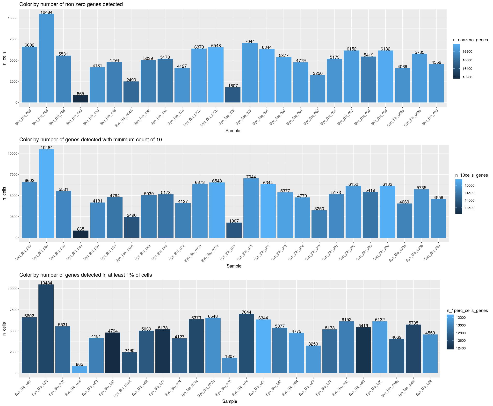
cat("\n\n")cat("#### Diagnosis \n\n")Diagnosis
print(ggpubr::ggarrange(
  ggplot(syn_nest_diagnosis_main, aes(x = Diagnosis_main, y = n_cells, fill = n_nonzero_genes)) +  # Plot with values on top
    geom_bar(stat = "identity") +
    geom_text(aes(label = n_cells), vjust = 0) +
    labs(title = "Color by number of non zero genes detected") +
    theme(axis.text.x = element_text(angle = 45,hjust=1)),
  ggplot(syn_nest_diagnosis_main, aes(x = Diagnosis_main, y = n_cells, fill = n_10cells_genes)) +  # Plot with values on top
    geom_bar(stat = "identity") +
    geom_text(aes(label = n_cells), vjust = 0) +
    labs(title = "Color by number of genes detected with minimum count of 10") +
    theme(axis.text.x = element_text(angle = 45,hjust=1)),
  ggplot(syn_nest_diagnosis_main, aes(x = Diagnosis_main, y = n_cells, fill = n_1perc_cells_genes)) +  # Plot with values on top
    geom_bar(stat = "identity") +
    geom_text(aes(label = n_cells), vjust = 0) +
    labs(title = "Color by number of genes detected in at least 1% of cells") +
    theme(axis.text.x = element_text(angle = 45,hjust=1)), nrow = 3))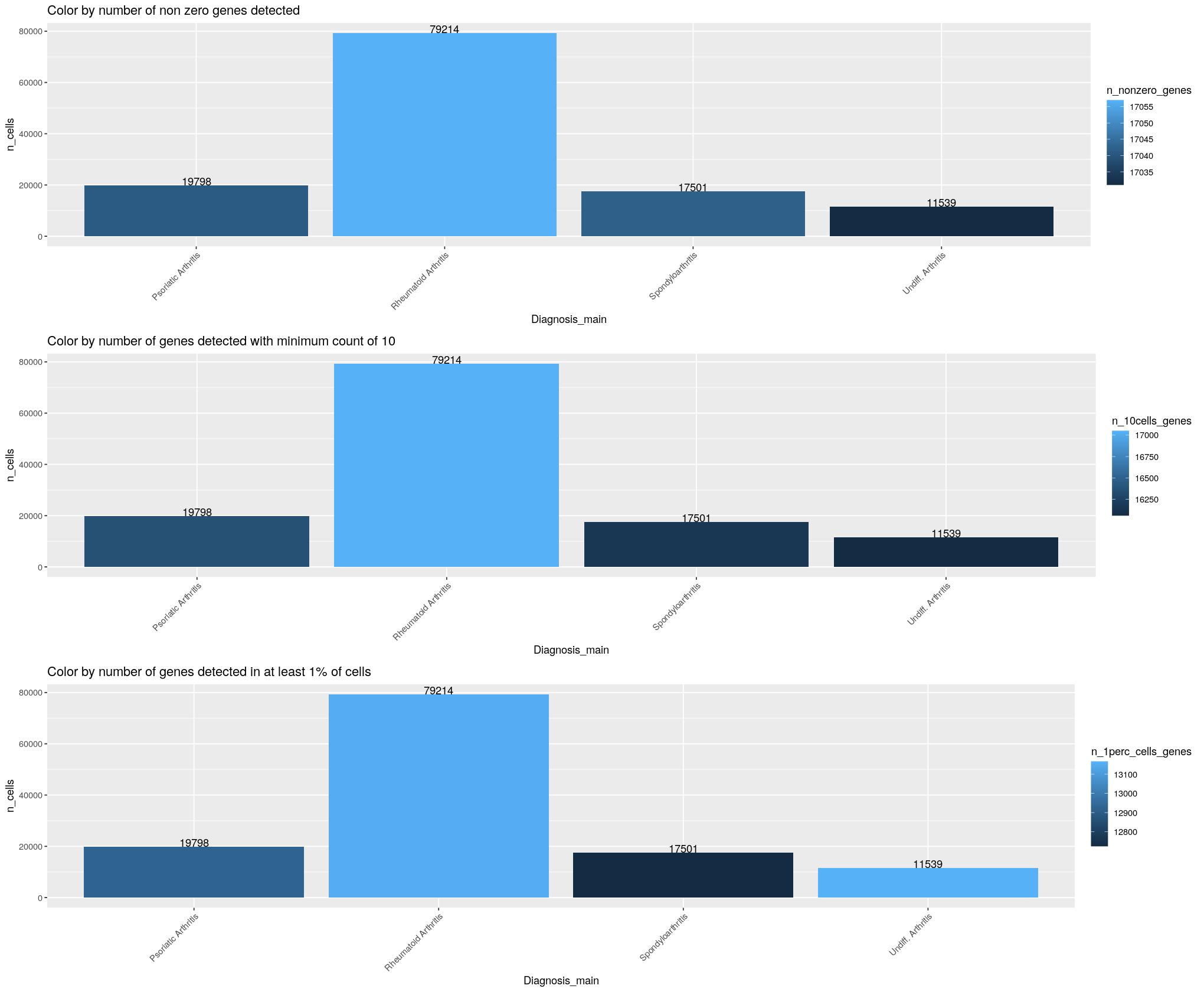
cat("\n\n")cat("#### Patient \n\n")Patient
print(ggpubr::ggarrange(
  ggplot(syn_nest_patient, aes(x = Patient, y = n_cells, fill = n_nonzero_genes)) +  # Plot with values on top
    geom_bar(stat = "identity") +
    geom_text(aes(label = n_cells), vjust = 0) +
    labs(title = "Color by number of non zero genes detected") +
    theme(axis.text.x = element_text(angle = 45,hjust=1)),
  ggplot(syn_nest_patient, aes(x = Patient, y = n_cells, fill = n_10cells_genes)) +  # Plot with values on top
    geom_bar(stat = "identity") +
    geom_text(aes(label = n_cells), vjust = 0) +
    labs(title = "Color by number of genes detected with minimum count of 10") +
    theme(axis.text.x = element_text(angle = 45,hjust=1)),
  ggplot(syn_nest_patient, aes(x = Patient, y = n_cells, fill = n_1perc_cells_genes)) +  # Plot with values on top
    geom_bar(stat = "identity") +
    geom_text(aes(label = n_cells), vjust = 0) +
    labs(title = "Color by number of genes detected in at least 1% of cells") +
    theme(axis.text.x = element_text(angle = 45,hjust=1)), nrow = 3))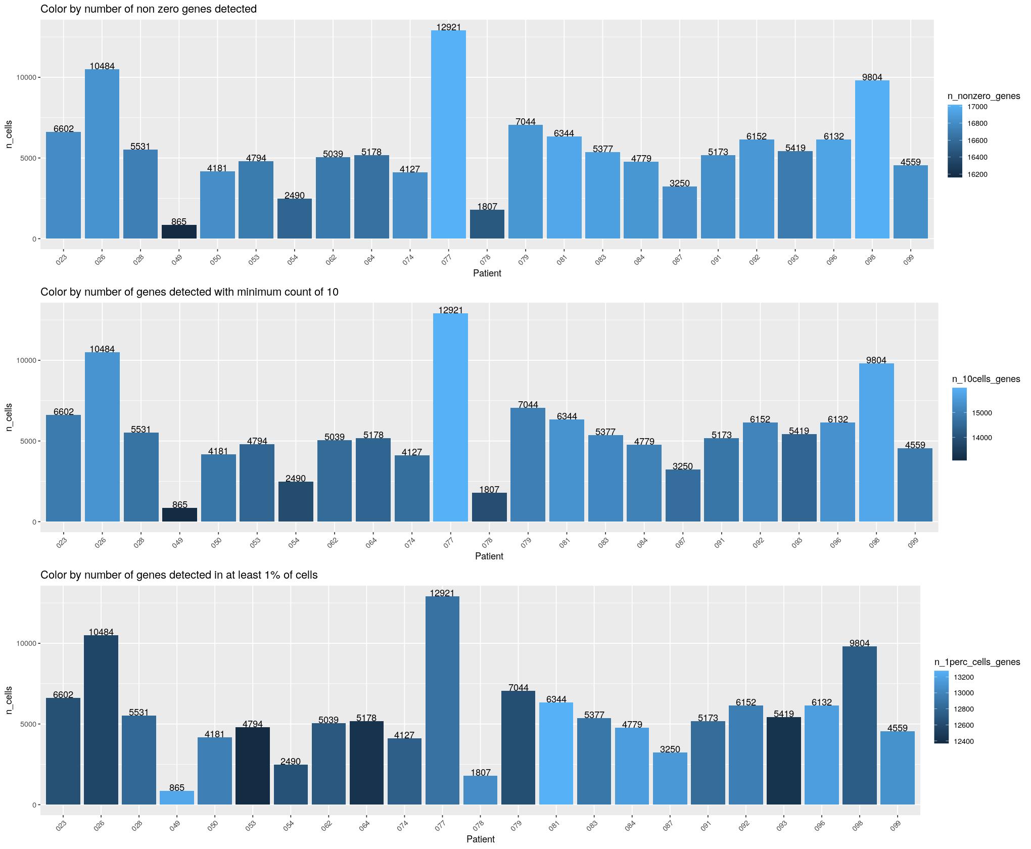
cat("\n\n")cat("### {-}")scuttle
Quality metrics per cell using scuttle.
is.mito <- grepl("\\.mt-", rownames(syn_sce_tidy), ignore.case = TRUE)
bpstart(bpparam)
syn_sce_tidy <-
  syn_sce_tidy %>%
      addPerCellQC(subsets = list(Mito = is.mito, genes = !is.mito), percent_top=c(50,100,200,500), BPPARAM=bpparam) %>%
      mutate(high_mitochondrion = isOutlier(subsets_Mito_percent, nmads=3, type = "higher", batch = Sample,
                                            subset = !(syn_sce_tidy$Sample %in% c("Syn_Bio_026","Syn_Bio_028","Syn_Bio_050","Syn_Bio_077a","Syn_Bio_098a","Syn_Bio_099"))),
             total_counts_drop = isOutlier(sum, nmads = 3, type = "both", log = TRUE, batch = Sample),
             total_counts_drop_fix = sum < 750,
             total_detected_drop = isOutlier(detected, nmads = 3, type = "both", log = TRUE, batch = Sample),
             to_exclude = high_mitochondrion | total_counts_drop | total_counts_drop_fix | total_detected_drop
      )
bpstop(bpparam)
syn_sce_tidy %>%
plotColData(x="Sample", y="subsets_Mito_percent", colour_by="to_exclude") +
theme(axis.text.x = element_text(angle = 90)) +
labs(x="", y="Percentage mito counts")+
ggtitle("Subset of mitochondrial genes in percent")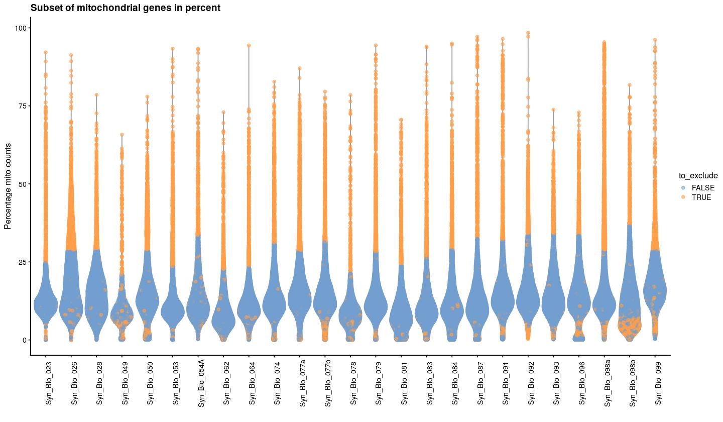
percentage mitochondrial counts per sample, each dot is a cell
cat("### Mito vs. Total {.tabset}\n\n")Mito vs. Total
cat("#### Color by exclude\n\n")Color by exclude
print(syn_sce_tidy %>%
  ggplot(aes(x=total, y=subsets_genes_detected, color=to_exclude)) +
    geom_point() +
    facet_wrap(~Sample, nrow=4) +
    labs(y="number of genes", x="total counts") +
    ggtitle("Total gene expression count vs. detected mitochondrial genes") +
    scale_x_log10() +
    scale_y_log10() +
    geom_density_2d(colour="black"))
Warning: stat_contour(): Zero contours were generatedWarning in min(x): no non-missing arguments to min; returning InfWarning in max(x): no non-missing arguments to max; returning -Inf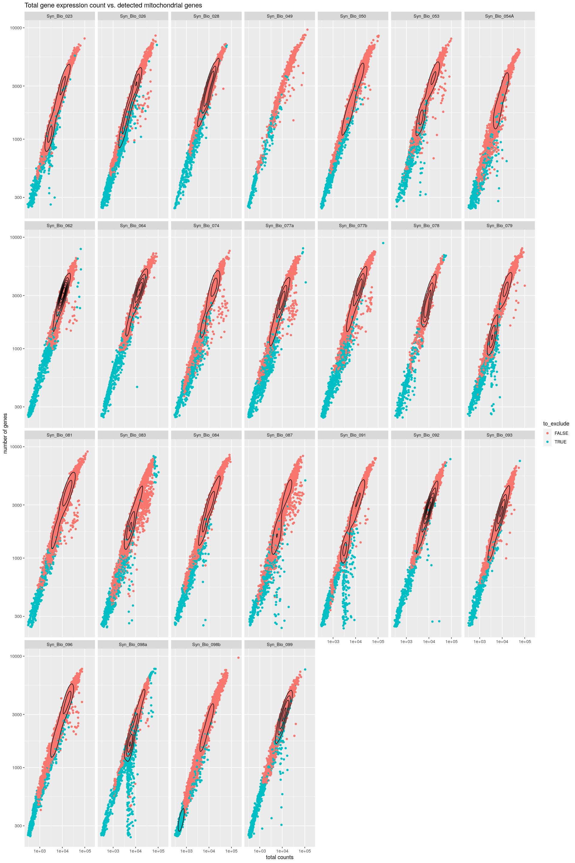
cat("\n\n")cat("#### Color by Mito\n\n")Color by Mito
print(syn_sce_tidy %>%
  ggplot(aes(x=total, y=subsets_genes_detected, color=subsets_Mito_percent)) +
    scale_color_gradient(low = "yellow", high = "darkred") +
    geom_point() +
    facet_wrap(~Sample, nrow=4) +
    labs(y="number of genes", x="total counts") +
    ggtitle("Total gene expression count vs. detected mitochondrial genes") +
    scale_x_log10() +
    scale_y_log10() +
    geom_density_2d(colour="black"))
Warning: stat_contour(): Zero contours were generatedWarning in min(x): no non-missing arguments to min; returning InfWarning in max(x): no non-missing arguments to max; returning -Inf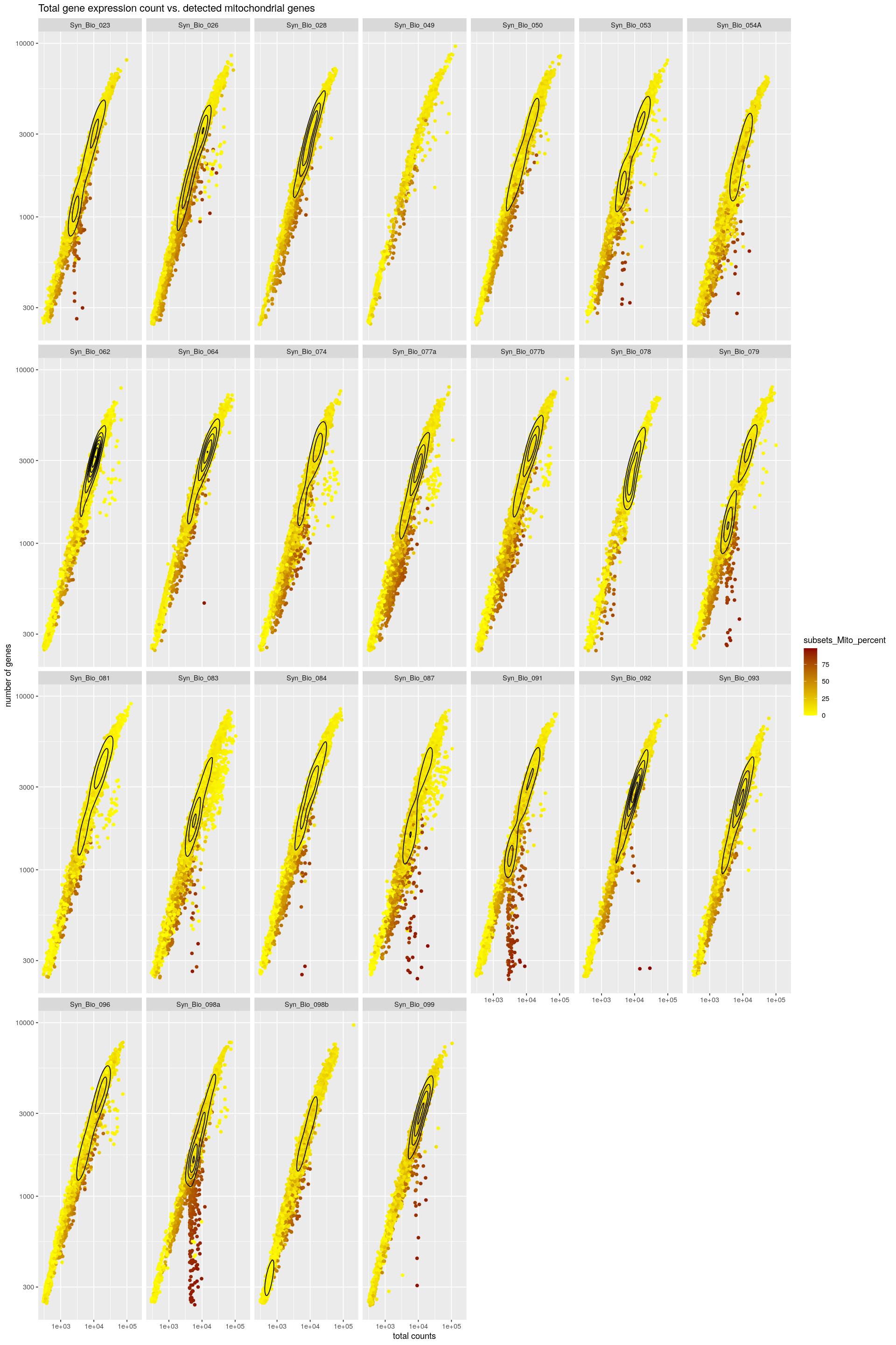
cat("\n\n")cat("### {-}")syn_sce_tidy %>%
plotColData(x=I(log(colData(syn_sce_tidy)$total)),
y="subsets_Mito_percent",
colour_by="to_exclude",
point_size=0.5,
point_alpha=0.5) +
ggtitle("Total gene expression values vs Total mitochondrial gene expression values") +
labs(x="log(Total counts)", y="Percentage mito counts") +
facet_wrap(~syn_sce_tidy$Sample, nrow = 5) +
theme(legend.position = c(0.92,0.97), legend.background = element_rect(color="grey",fill = "white"), legend.margin = margin(10,10,10,10))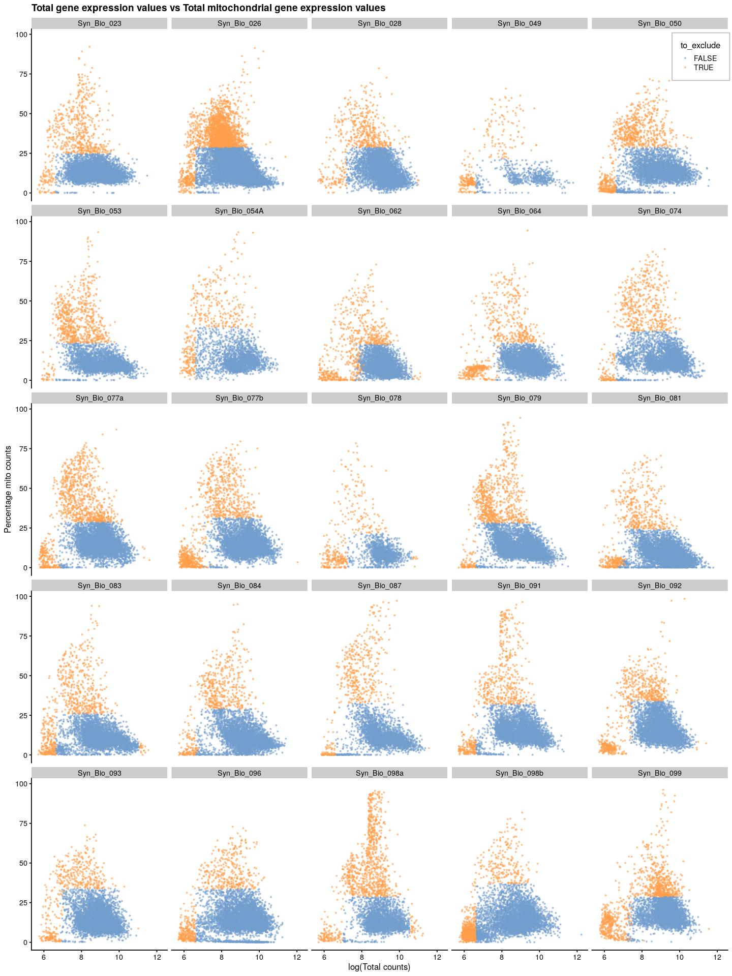
SampleQC
Another cell quality method, called SampleQC.
library(SampleQC)
syn_sce_tidy$patient_id <- syn_sce_tidy$Sample
syn_sce_tidy$sample_id <- syn_sce_tidy$Sample

rownames(syn_sce_tidy) <- rowData(syn_sce_tidy)$Symbol
qc_dt   = suppressWarnings(make_qc_dt(syn_sce_tidy))

qc_names        = c('log_counts', 'log_feats', 'logit_mito')
annots_disc     = c('patient_id')
annots_cont     = NULL

tmp <- capture.output(qc_obj <-
  calc_pairwise_mmds(qc_dt,
                                  qc_names,
                                  annots_disc=annots_disc,
                                  annots_cont=annots_cont,
                                  n_cores=n_workers,
                                  seed = 123)
  )
sample-level parts of SampleQC: calculating 300 sample-sample MMDs: clustering samples using MMD values calculating MDS embedding calculating UMAP embedding adding annotation variables constructing SampleQC objecttmp <- capture.output(qc_obj <-
fit_sampleqc(qc_obj,
K_list=rep(1, get_n_groups(qc_obj)),
bp_seed = 123)
)max 50 EM iterations:
.
took 1 iterationsmax 50 EM iterations:
.
took 1 iterations
max 50 EM iterations:
.
took 1 iterationsoutliers_dt = get_outliers(qc_obj)
# sort and add
colData(syn_sce_tidy)$SampleQC_outlier[match(outliers_dt$cell_id, colnames(syn_sce_tidy))] <- outliers_dt$outlier
syn_sce_tidy <- syn_sce_tidy %>%
dplyr::mutate(SampleQC_outlier_mito = syn_sce_tidy$SampleQC_outlier | syn_sce_tidy$high_mitochondrion | syn_sce_tidy$total_counts_drop_fix)
# comparison to scuttle
table(scuttle=syn_sce_tidy$to_exclude, SampleQC=syn_sce_tidy$SampleQC_outlier) SampleQC
scuttle FALSE TRUE
FALSE 102655 6152
TRUE 8338 10907# comparison to scuttle, add mito limit to SampleQC
table(scuttle=syn_sce_tidy$to_exclude, SampleQC=syn_sce_tidy$SampleQC_outlier_mito) SampleQC
scuttle FALSE TRUE
FALSE 102655 6152
TRUE 103 19142syn_sce_tidy %>%
plotColData(x="Sample", y="subsets_Mito_percent", colour_by="SampleQC_outlier_mito") +
labs(x="", y="Percentage mito counts")+
theme(axis.text.x = element_text(angle = 90)) +
ggtitle("Subset of mitochondrial genes in percent")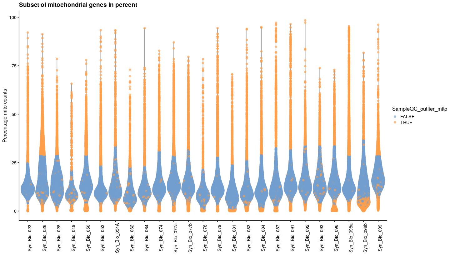
cat("### Mito vs. Total {.tabset}\n\n")Mito vs. Total
cat("#### Color by exclude\n\n")Color by exclude
sfig1a1 <- syn_sce_tidy %>%
  dplyr::select(total, subsets_genes_detected, SampleQC_outlier_mito, Sample) %>%
  ggplot(aes(x=total, y=subsets_genes_detected, color=SampleQC_outlier_mito)) +
    geom_point(size=0.5) +
    facet_wrap(~Sample, nrow=4) +
    labs(title = "Total gene expression count vs. number of detected genes",
         x = "Total counts", y = "Number of genes",
         colour = "Exclude cell") +
    scale_x_log10() +
    scale_y_log10() +
    geom_density_2d(colour="black", alpha=0.5) +
    main_plot_theme()
tidySingleCellExperiment says: Key columns are missing. A data frame is returned for independent data analysis.print(sfig1a1)Warning: stat_contour(): Zero contours were generatedWarning in min(x): no non-missing arguments to min; returning InfWarning in max(x): no non-missing arguments to max; returning -Inf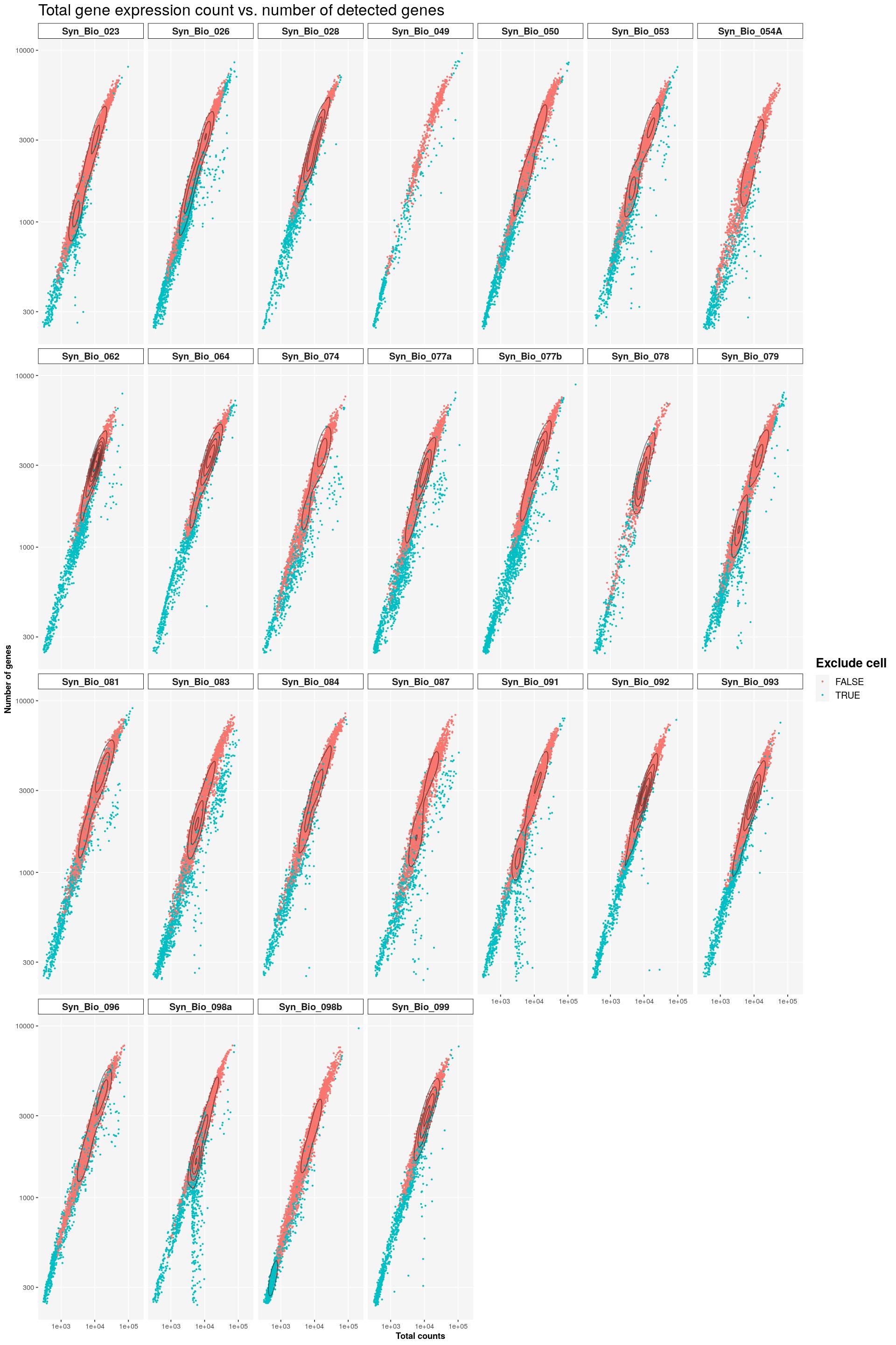
cat("\n\n")cat("#### Color by Mito\n\n")Color by Mito
sfig1a2 <- syn_sce_tidy %>%
  dplyr::select(total, subsets_genes_detected, subsets_Mito_percent, Sample) %>%
  ggplot(aes(x=total, y=subsets_genes_detected, color=subsets_Mito_percent)) +
    scale_color_gradient(low = "yellow", high = "darkred") +
    geom_point(size=0.5) +
    facet_wrap(~Sample, nrow=4) +
    labs(title = "Total gene expression count vs. number of detected genes",
       x = "Total counts", y = "Number of genes",
       colour = "Percentage\nMitochondrial\ncounts") +
    scale_x_log10() +
    scale_y_log10() +
    geom_density_2d(colour="black", alpha=0.5) +
    main_plot_theme()
tidySingleCellExperiment says: Key columns are missing. A data frame is returned for independent data analysis.print(sfig1a2)Warning: stat_contour(): Zero contours were generatedWarning in min(x): no non-missing arguments to min; returning InfWarning in max(x): no non-missing arguments to max; returning -Inf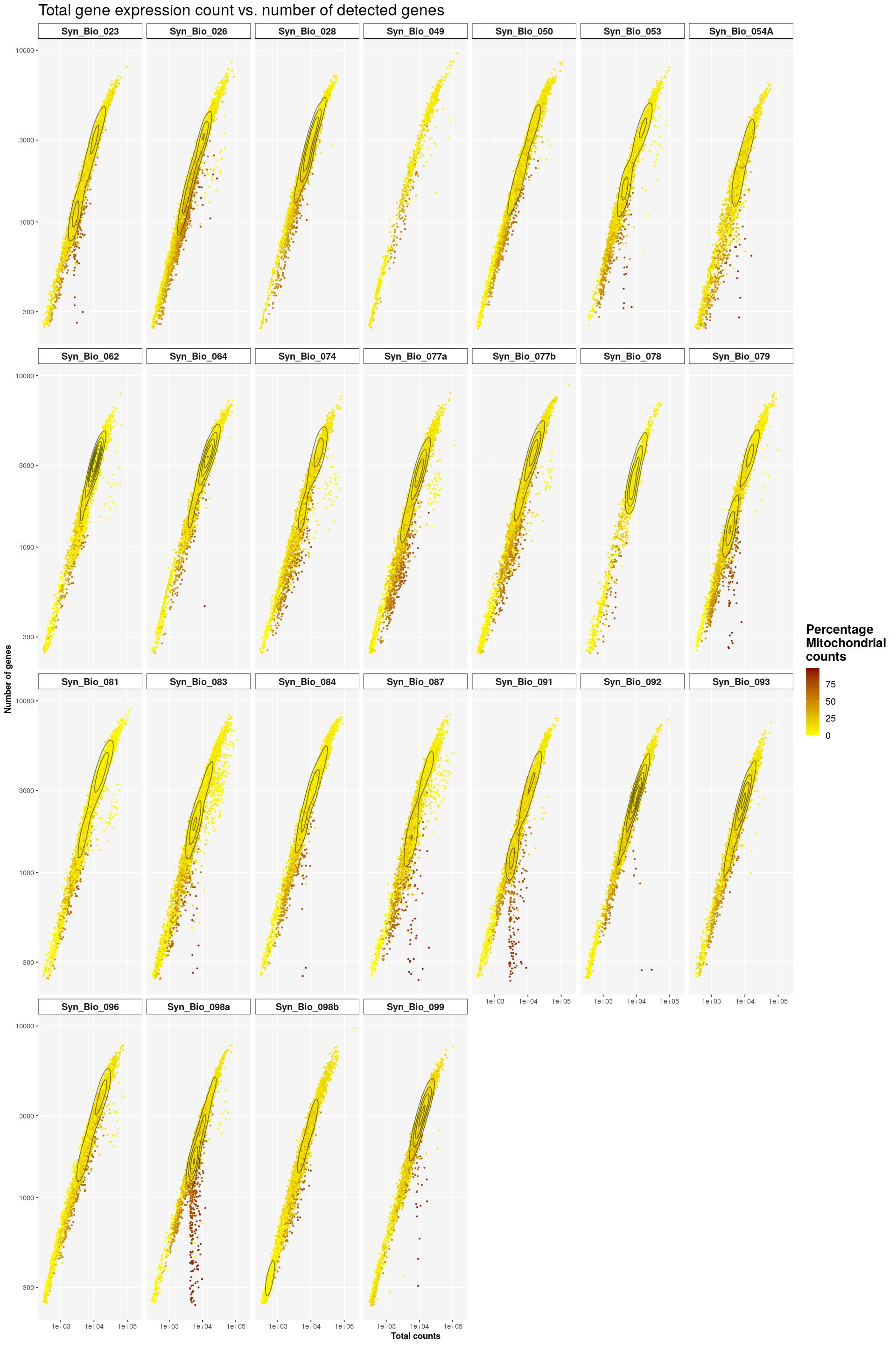
cat("\n\n")cat("### {-}")syn_sce_tidy %>%
plotColData(x=I(log(colData(syn_sce_tidy)$total)),
y="subsets_Mito_percent",
colour_by="SampleQC_outlier_mito",
point_size=0.5,
point_alpha=0.5) +
ggtitle("Total gene expression values vs Total mitochondrial gene expression values") +
labs(x="log(Total counts)", y="Percentage mito counts") +
facet_wrap(~syn_sce_tidy$Sample, nrow = 5) +
theme(legend.position = c(0.92,0.97), legend.background = element_rect(color="grey",fill = "white"), legend.margin = margin(10,10,10,10))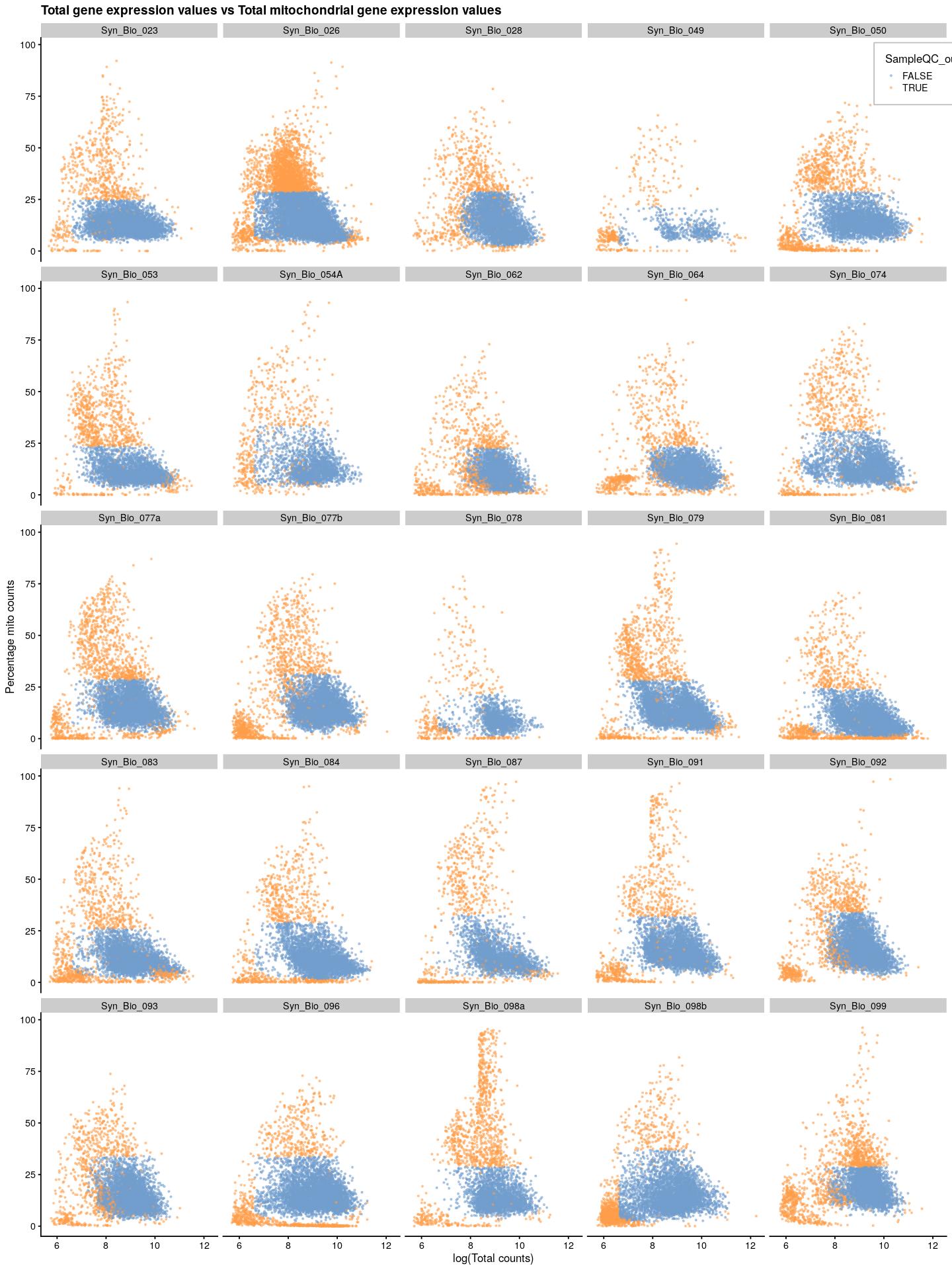
dim(syn_sce_tidy)[1] 17057 128052syn_sce_tidy_filtered <- syn_sce_tidy %>% filter(!SampleQC_outlier_mito)
dim(syn_sce_tidy_filtered)[1] 17057 102758syn_sce_tidy_filtered <- syn_sce_tidy_filtered[rowSums(counts(syn_sce_tidy_filtered) > 0) > 10, ]
dim(syn_sce_tidy_filtered)[1] 17057 102758prepare abundance plot data.
syn_nest_Sample <- syn_sce_tidy_filtered %>%
  nest(data=-Sample) %>%
  mutate(n_cells = purrr::map_dbl(data, ~ dim(.x)[2]),
         n_nonzero_genes = purrr::map_dbl(data, ~ sum(rowSums(counts(.x) > 0) > 0)),
         n_10cells_genes = purrr::map_dbl(data, ~ sum(rowSums(counts(.x) > 0) > 10)),
         n_1perc_cells_genes = purrr::map_dbl(data, ~ sum(rowSums(counts(.x) > 0) > ceiling(dim(.x)[2]/100))))

syn_nest_diagnosis <- syn_sce_tidy_filtered %>%
  nest(data=-Diagnosis_main) %>%
  mutate(n_cells = purrr::map_dbl(data, ~ dim(.x)[2]),
         n_nonzero_genes = purrr::map_dbl(data, ~ sum(rowSums(counts(.x) > 0) > 0)),
         n_10cells_genes = purrr::map_dbl(data, ~ sum(rowSums(counts(.x) > 0) > 10)),
         n_1perc_cells_genes = purrr::map_dbl(data, ~ sum(rowSums(counts(.x) > 0) > ceiling(dim(.x)[2]/100))))
plot abundances, colored by number of genes detected.
cat("### Number of Cells {.tabset}\n\n")Number of Cells
cat("#### Unique Samples \n\n")Unique Samples
sfig1b1 <- ggpubr::ggarrange(
  ggplot(syn_nest_Sample, aes(x = Sample, y = n_cells, fill = n_nonzero_genes)) +  # Plot with values on top
    geom_bar(stat = "identity") +
    geom_text(aes(label = n_cells), vjust = 0) +
    labs(title = "", x="", fill="Number of genes", y="Number of cells") +
  main_plot_theme() +
    theme(axis.text.x = element_text(angle = 45,hjust=1), axis.ticks.x=element_blank(),
          legend.position = c(1.1,0.5),plot.margin = margin(0,110,0,0)),
  ggplot(syn_nest_Sample, aes(x = Sample, y = n_cells, fill = n_1perc_cells_genes)) +  # Plot with values on top
    geom_bar(stat = "identity") +
    geom_text(aes(label = n_cells), vjust = 0) +
    labs(title = "", x="",
         fill="Number of genes\nin at least \n1% of cells",  y="Number of cells") +
    theme(axis.text.x = element_text(angle = 45,hjust=1), axis.ticks.x=element_blank(),
          legend.position = c(1.1,0.5),plot.margin = margin(0,110,0,0)) +
  main_plot_theme(),
  nrow = 2)
print(sfig1b1)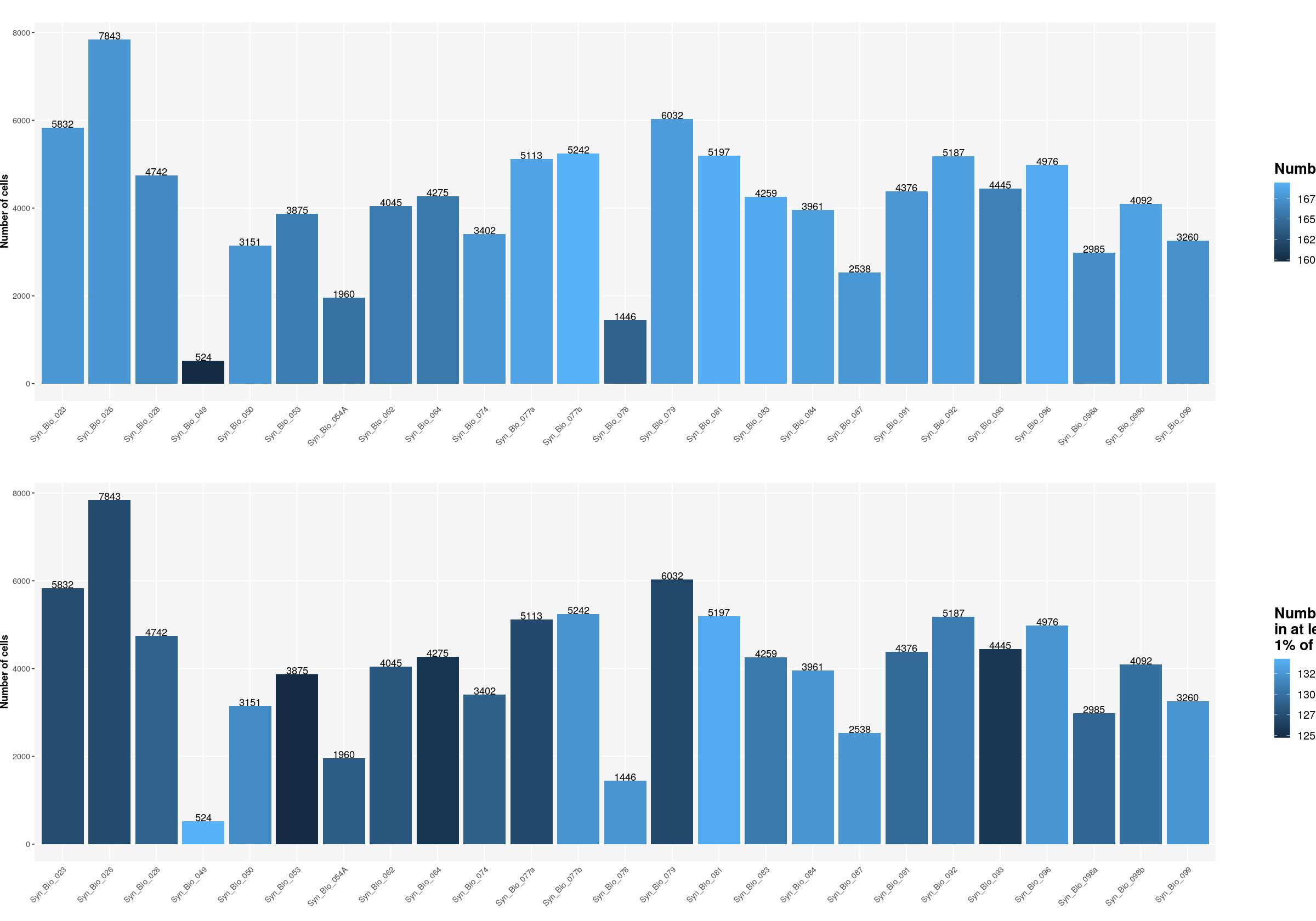
| Version | Author | Date |
|---|---|---|
| 7d99571 | Reto Gerber | 2022-03-21 |
cat("\n\n")cat("#### Diagnosis \n\n")Diagnosis
sfig1b2 <- ggpubr::ggarrange(
  ggplot(syn_nest_diagnosis, aes(x = Diagnosis_main, y = n_cells, fill = n_nonzero_genes)) +  # Plot with values on top
    geom_bar(stat = "identity") +
    geom_text(aes(label = n_cells), vjust = 0) +
    labs(title = "", x="", fill="Number of genes", y="Number of cells") +
  main_plot_theme() +
    theme(axis.text.x = element_text(angle = 45,hjust=1), axis.ticks.x=element_blank(),
          legend.position = c(1.1,0.5),plot.margin = margin(0,110,0,0)),
  ggplot(syn_nest_diagnosis, aes(x = Diagnosis_main, y = n_cells, fill = n_1perc_cells_genes)) +  # Plot with values on top
    geom_bar(stat = "identity") +
    geom_text(aes(label = n_cells), vjust = 0) +
    labs(title = "", x="",
         fill="Number of genes\nin at least \n1% of cells",  y="Number of cells") +
    theme(axis.text.x = element_text(angle = 45,hjust=1), axis.ticks.x=element_blank(),
          legend.position = c(1.1,0.5),plot.margin = margin(0,110,0,0)) +
  main_plot_theme(),
  nrow = 2)
print(sfig1b2)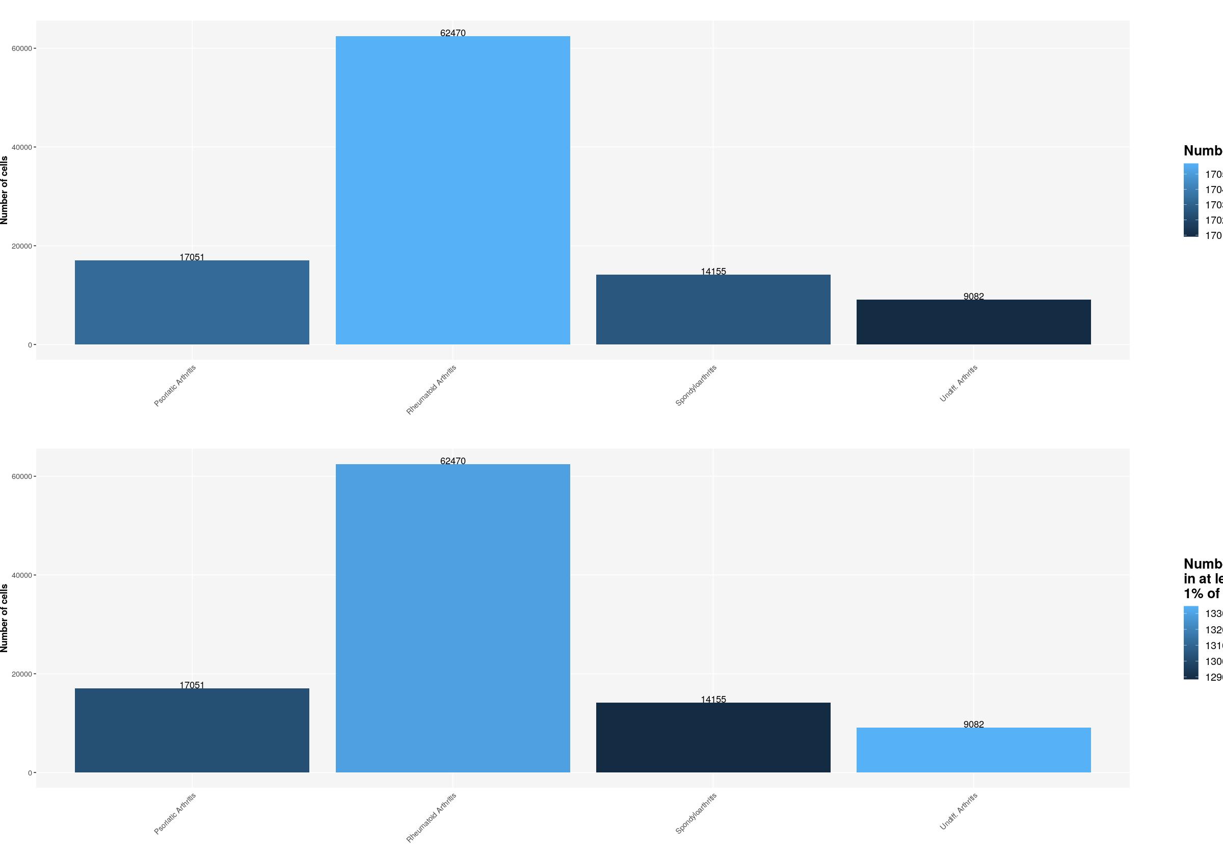
cat("\n\n")cat("### {-}")sfig1c1 <- syn_sce_tidy %>%
dplyr::select(total, Diagnosis_main) %>%
ggplot() +
geom_density(aes(log10(total), fill=Diagnosis_main, color=Diagnosis_main),alpha=0.3) +
scale_fill_manual(values=get_colors("diagnosis")[names(get_colors("diagnosis")) %in% unique(syn_sce_tidy$Diagnosis_main)]) +
scale_color_manual(values=get_colors("diagnosis")[names(get_colors("diagnosis")) %in% unique(syn_sce_tidy$Diagnosis_main)]) +
main_plot_theme()tidySingleCellExperiment says: Key columns are missing. A data frame is returned for independent data analysis.sfig1c1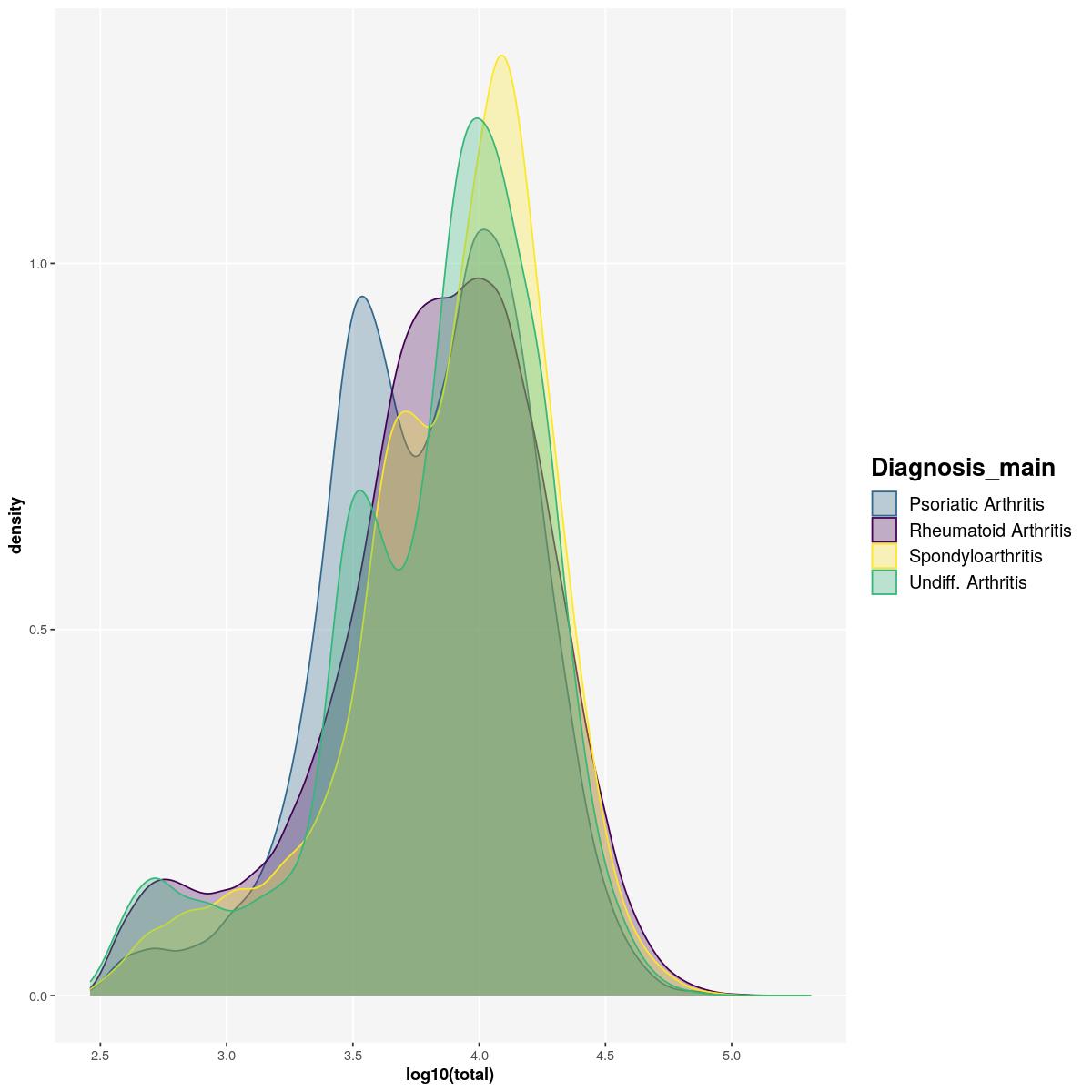
sfig1c2 <- syn_sce_tidy  %>%
  dplyr::select(total, Sample, Diagnosis_main) %>%
  ggplot() +
  geom_density(aes(log10(total), fill=Sample, color=Sample),alpha=0.1) +
  scale_color_manual(values=sample_cols(unique(syn_sce_tidy$Sample), n_split=5)) +
  scale_fill_manual(values=sample_cols(unique(syn_sce_tidy$Sample), n_split=5))+
  facet_grid(rows = vars(Diagnosis_main)) +
  main_plot_theme()
tidySingleCellExperiment says: Key columns are missing. A data frame is returned for independent data analysis.sfig1c2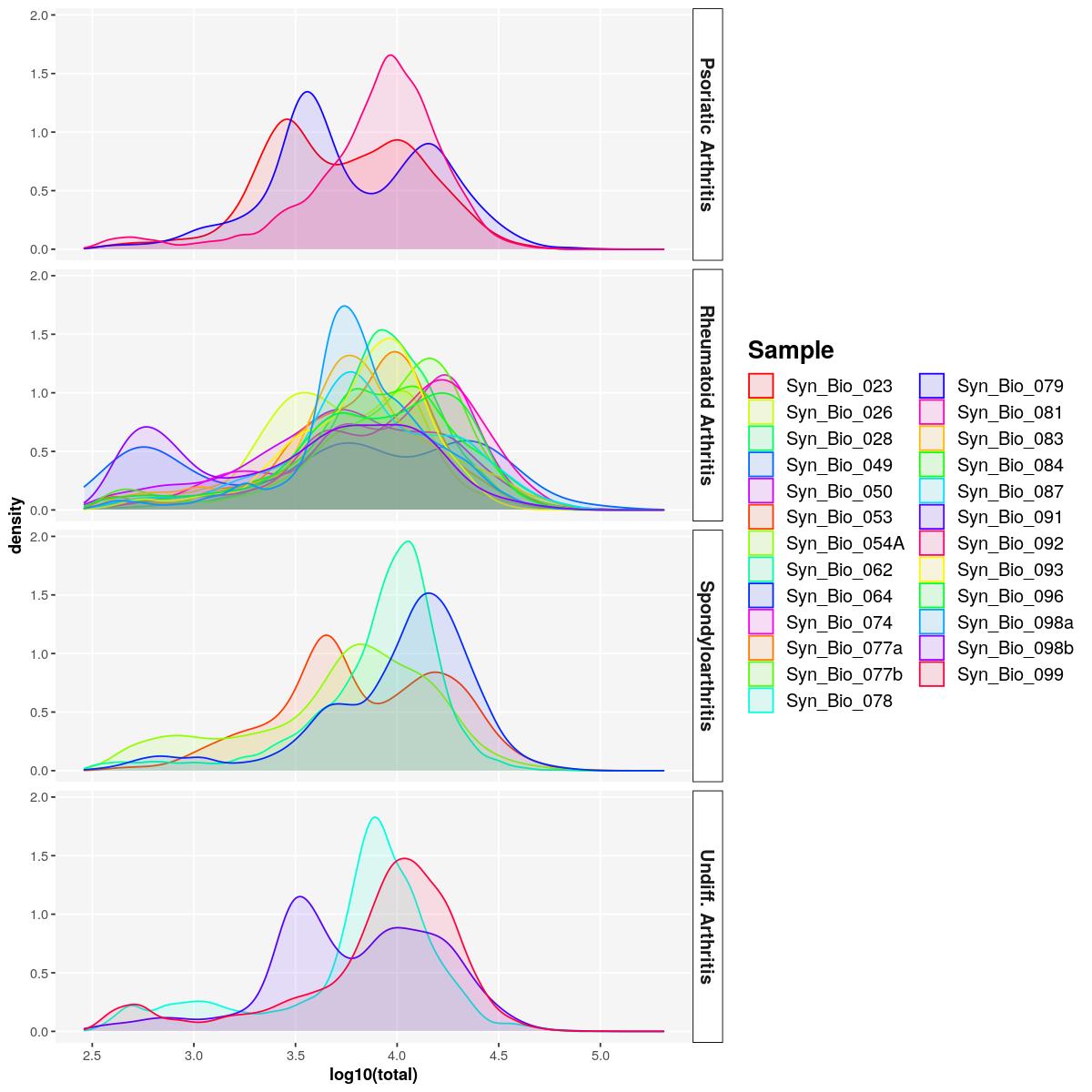
sfig1d1 <- syn_sce_tidy %>%
  dplyr::select(detected, Diagnosis_main) %>%
  ggplot() +
  geom_density(aes(log10(detected), fill=Diagnosis_main),alpha=0.5) +
  labs(x="log10(Number of genes)")+
  main_plot_theme()
tidySingleCellExperiment says: Key columns are missing. A data frame is returned for independent data analysis.sfig1d1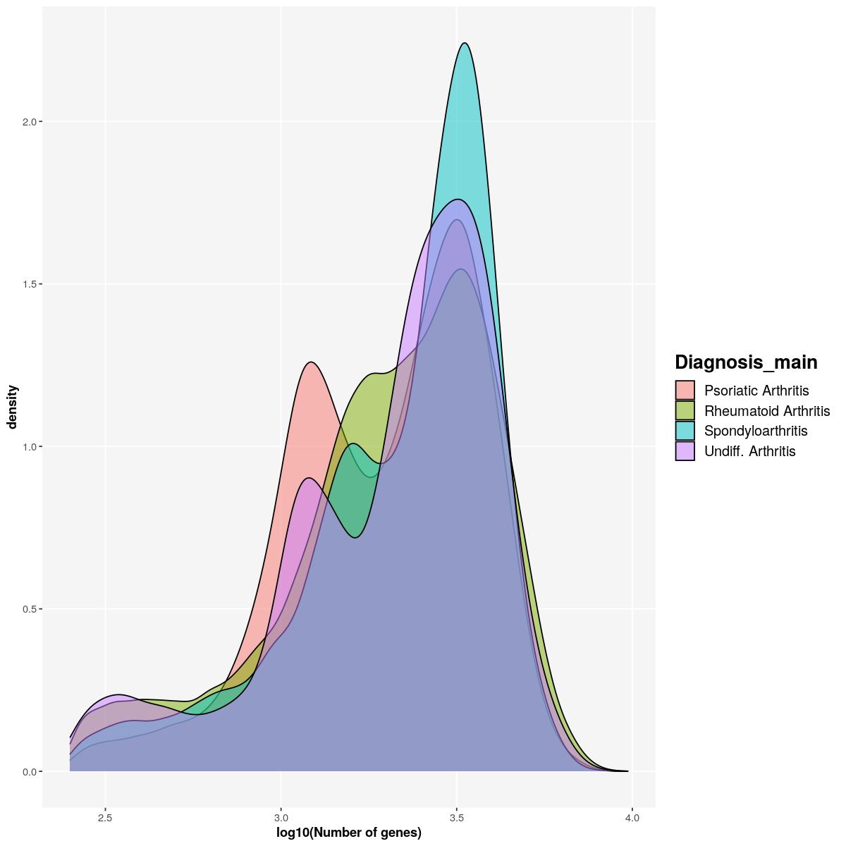
sfig1d2 <- syn_sce_tidy %>%
  dplyr::select(detected, Diagnosis_main,Sample) %>%
  ggplot() +
  geom_density(aes(log10(detected), fill=Sample, color=Sample),alpha=0.1) +
  labs(x="log10(Number of genes)")+
  scale_color_manual(values=sample_cols(unique(syn_sce_tidy$Sample), n_split=5)) +
  scale_fill_manual(values=sample_cols(unique(syn_sce_tidy$Sample), n_split=5))+
  facet_grid(rows = vars(Diagnosis_main)) +
  main_plot_theme()
tidySingleCellExperiment says: Key columns are missing. A data frame is returned for independent data analysis.sfig1d2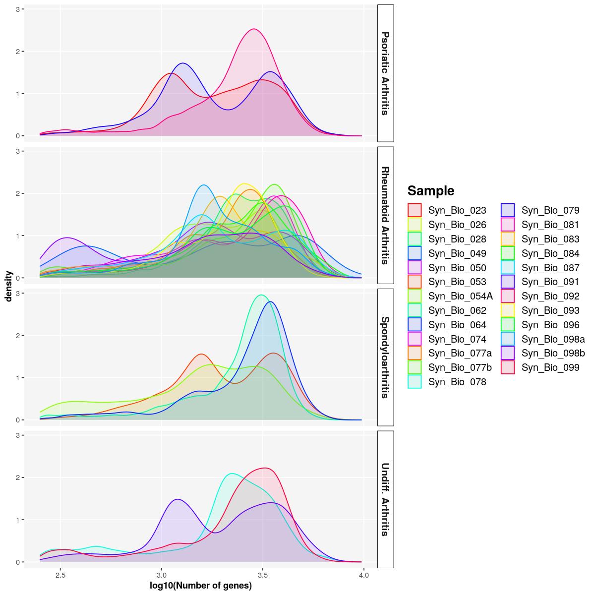
Normalization
Histogram of library size factors. Also quick clustering and computation of sum factors for better normalization (i.e. corrected for variability between celltypes).
bpstart(bpparam)
lib.sce <- syn_sce_tidy_filtered %>%  librarySizeFactors(BPPARAM=bpparam)
bpstop(bpparam)
hist(log10(lib.sce), xlab="Log10[Size factor]", col='grey80')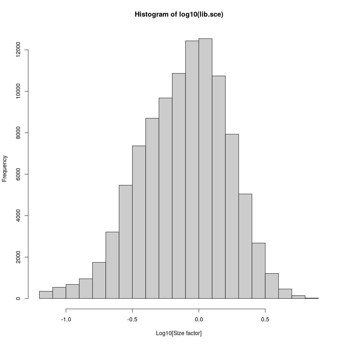
bpstart(bpparam)
clust.sce <- syn_sce_tidy_filtered %>%  quickCluster(BPPARAM=bpparam)
bpstop(bpparam)
bpstart(bpparam)
syn_sce_tidy_filtered <- syn_sce_tidy_filtered %>%  computeSumFactors(cluster=clust.sce,BPPARAM=bpparam)
bpstop(bpparam)
plot(lib.sce, sizeFactors(syn_sce_tidy_filtered), xlab="Library size factor",
    ylab="Deconvolution size factor", log='xy', pch=16,
    col=as.integer(factor(clust.sce)))
abline(a=0, b=1, col="red")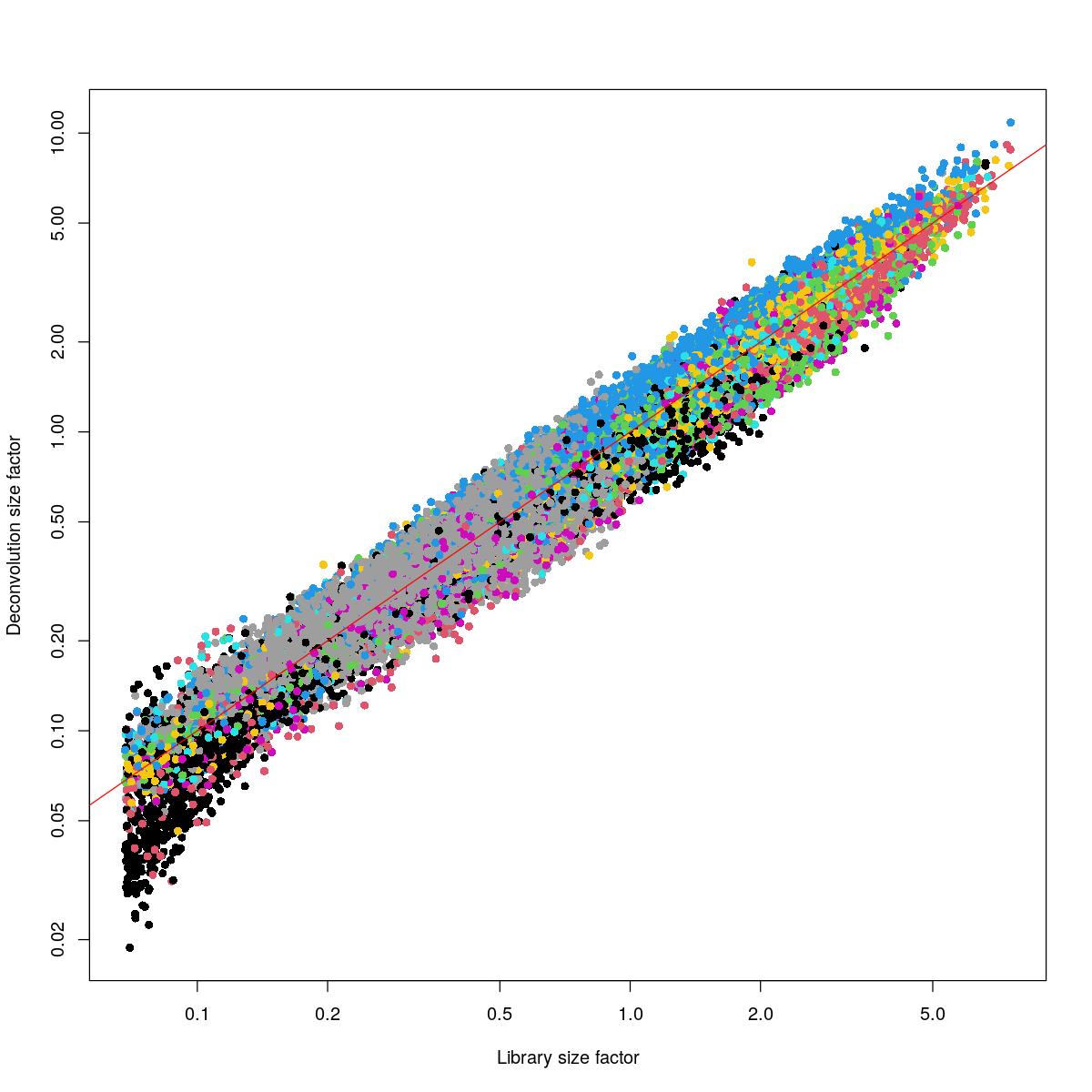
plot(lib.sce, sizeFactors(syn_sce_tidy_filtered), xlab="Library size factor",
    ylab="Deconvolution size factor", log='xy', pch=16,
    col=as.integer(factor(syn_sce_tidy_filtered$Sample)),
    main="Deconvolution factors for individual clusters")

abline(a=0, b=1, col="red")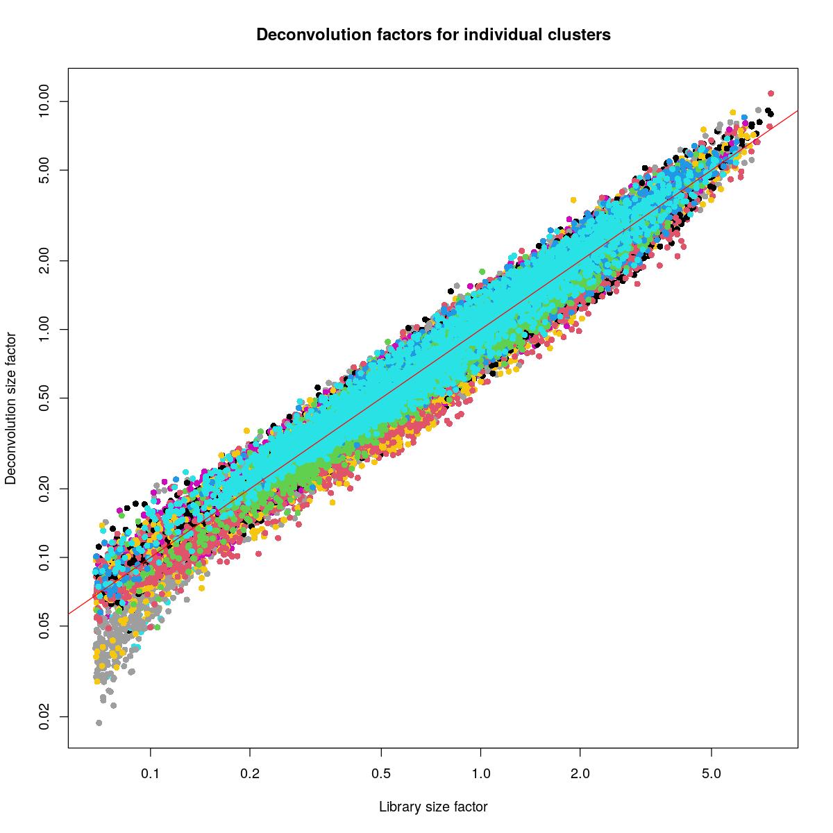
Apply normalization, run PCA.
syn_sce_tidy_filtered <- syn_sce_tidy_filtered %>%
  logNormCounts() %>%
  runPCA()
size_fac_for_plotting <- I(librarySizeFactors(syn_sce_tidy_filtered))
table(factor(size_fac_for_plotting > 3, labels = c("<= 3", "> 3")))/length(size_fac_for_plotting)
      <= 3        > 3
0.97795792 0.02204208
size_fac_for_plotting[size_fac_for_plotting > 3] <- 3
plotPCA(syn_sce_tidy_filtered, colour_by=size_fac_for_plotting, ncomponents=2) + ggtitle(paste("Size factors"))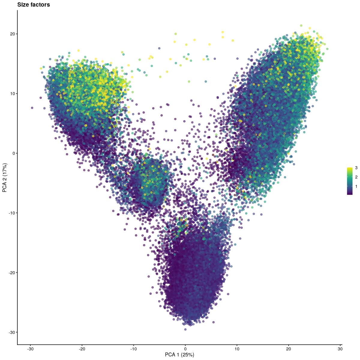
plot PCA, colored by size factor.
pca_pl_ls <- list()
for(pa_id in unique(syn_sce_tidy_filtered$patient_ID)){
  pat_filt <- syn_sce_tidy_filtered$patient_ID==pa_id
  pca_pl_ls[[pa_id]] <- plotPCA(syn_sce_tidy_filtered %>% filter(pat_filt), colour_by=size_fac_for_plotting[pat_filt], ncomponents=2) + ggtitle(paste("Size factor for Patient:",pa_id))
}
n_sam <- length(pca_pl_ls)
cat("### By Patient {.tabset}\n\n")
By Patient
for(i in seq_len(ceiling(n_sam/4))){
  pl_ind <- (((i-1)*4)+1):(((i)*4))
  pl_ind <- pl_ind[pl_ind <= n_sam]
  if(length(pl_ind) > 0){
    cat("#### Patients: ",paste(names(pca_pl_ls)[pl_ind]),"\n\n")
    print(ggpubr::ggarrange(plotlist=pca_pl_ls[pl_ind]))
    cat("\n\n")
  }
}
cat("### {-}")
tmpfilename <- paste0("syn_v",analysis_version,"_sce_filtered",dplyr::if_else(remove_low_quality_samples, "_invivo",""),".rds")
saveRDS(syn_sce_tidy_filtered, file = here::here("output",tmpfilename))2nd Part: HVG selection, Dimensionality reduction
Supplementary Figure 1
saveRDS(list(sfig1a1=sfig1a1, sfig1a2=sfig1a2,
             sfig1b1=sfig1b1, sfig1b2=sfig1b2,
             syn_nest_Sample=syn_nest_Sample, syn_nest_diagnosis=syn_nest_diagnosis,
             sfig1c1=sfig1c1, sfig1c2=sfig1c2,
             sfig1d1=sfig1d1, sfig1d2=sfig1d2),
        file = here::here("output",paste0("syn_v",analysis_version,"_sfig1.rds")))
ggpubr::ggarrange(
ggpubr::ggarrange(sfig1a1,sfig1a2, ncol = 2),
ggpubr::ggarrange(sfig1b1, sfig1b2, ncol=2),
ggpubr::ggarrange(sfig1c1, sfig1c2, ncol=2),
ggpubr::ggarrange(sfig1d1, sfig1d2, ncol=2),
ncol = 1, nrow = 4,labels = "AUTO"
)Warning: stat_contour(): Zero contours were generatedWarning in min(x): no non-missing arguments to min; returning InfWarning in max(x): no non-missing arguments to max; returning -InfWarning: stat_contour(): Zero contours were generatedWarning in min(x): no non-missing arguments to min; returning InfWarning in max(x): no non-missing arguments to max; returning -Inf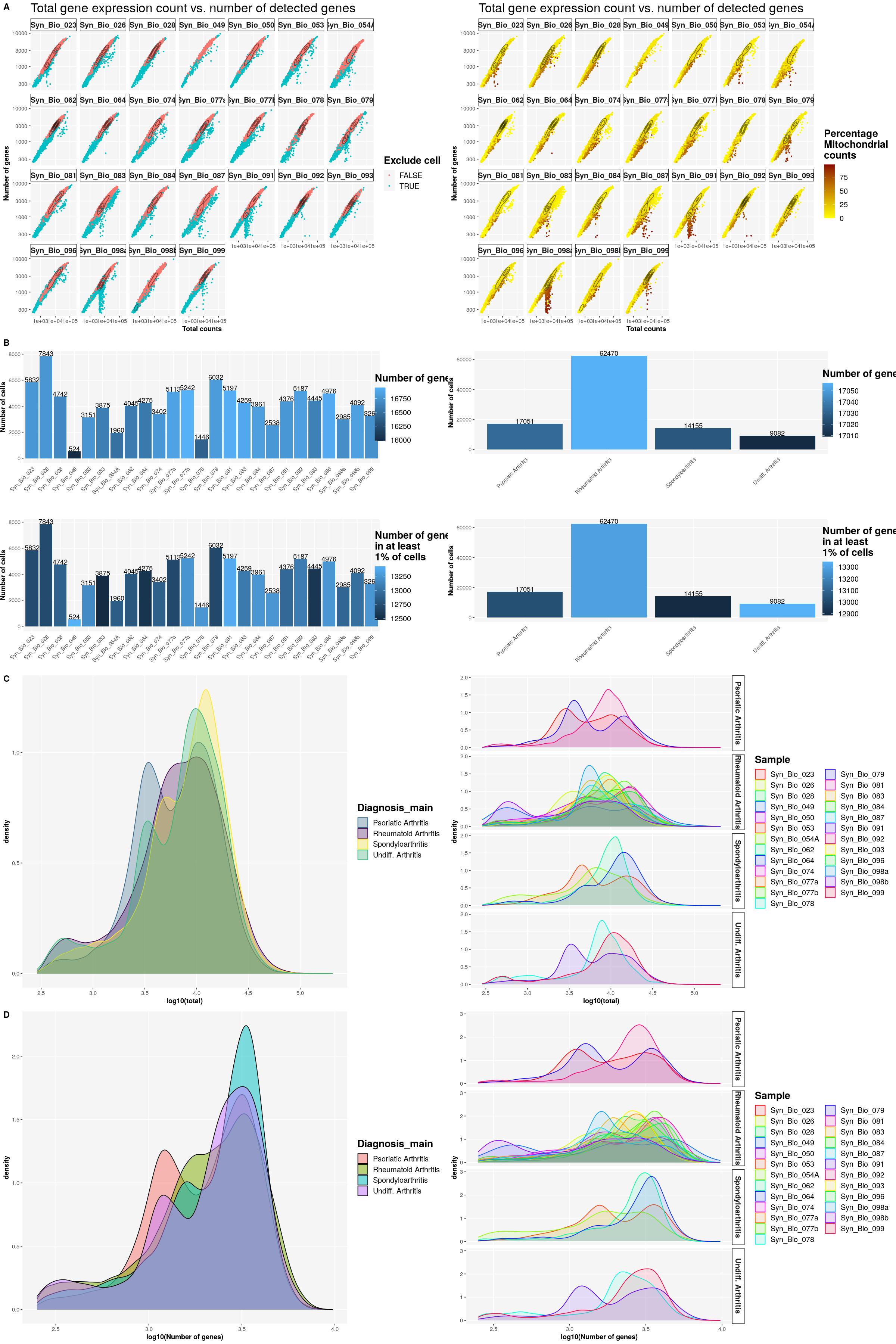
sessionInfo()R version 4.0.3 (2020-10-10)
Platform: x86_64-pc-linux-gnu (64-bit)
Running under: Ubuntu 20.04 LTS
Matrix products: default
BLAS/LAPACK: /usr/lib/x86_64-linux-gnu/openblas-pthread/libopenblasp-r0.3.8.so
locale:
[1] LC_CTYPE=en_US.UTF-8 LC_NUMERIC=C
[3] LC_TIME=en_US.UTF-8 LC_COLLATE=en_US.UTF-8
[5] LC_MONETARY=en_US.UTF-8 LC_MESSAGES=C
[7] LC_PAPER=en_US.UTF-8 LC_NAME=C
[9] LC_ADDRESS=C LC_TELEPHONE=C
[11] LC_MEASUREMENT=en_US.UTF-8 LC_IDENTIFICATION=C
attached base packages:
[1] parallel stats4 stats graphics grDevices utils datasets
[8] methods base
other attached packages:
[1] SampleQC_0.6.0 BiocParallel_1.24.1
[3] bluster_1.0.0 tidySingleCellExperiment_1.0.0
[5] ggbeeswarm_0.6.0 celldex_1.0.0
[7] scuttle_1.0.4 SingleR_1.4.1
[9] igraph_1.2.6 scran_1.18.7
[11] scater_1.18.6 SingleCellExperiment_1.12.0
[13] SummarizedExperiment_1.20.0 Biobase_2.50.0
[15] GenomicRanges_1.42.0 GenomeInfoDb_1.26.7
[17] IRanges_2.24.1 S4Vectors_0.28.1
[19] BiocGenerics_0.36.1 MatrixGenerics_1.2.1
[21] matrixStats_0.58.0 stringr_1.4.0
[23] purrr_0.3.4 ggplot2_3.3.3
[25] dplyr_1.0.4 workflowr_1.6.2
loaded via a namespace (and not attached):
[1] readxl_1.3.1 backports_1.2.1
[3] AnnotationHub_2.22.1 BiocFileCache_1.14.0
[5] lazyeval_0.2.2 splines_4.0.3
[7] digest_0.6.27 htmltools_0.5.1.1
[9] viridis_0.5.1 fansi_0.4.2
[11] magrittr_2.0.1 memoise_2.0.0
[13] mixtools_1.2.0 openxlsx_4.2.3
[15] limma_3.46.0 scDblFinder_1.4.0
[17] colorspace_2.0-0 blob_1.2.1
[19] rappdirs_0.3.3 haven_2.3.1
[21] xfun_0.21 crayon_1.4.1
[23] RCurl_1.98-1.2 jsonlite_1.7.2
[25] survival_3.2-7 glue_1.4.2
[27] gtable_0.3.0 zlibbioc_1.36.0
[29] XVector_0.30.0 DelayedArray_0.16.3
[31] kernlab_0.9-29 car_3.0-10
[33] BiocSingular_1.6.0 abind_1.4-5
[35] scales_1.1.1 mvtnorm_1.1-1
[37] DBI_1.1.1 edgeR_3.32.1
[39] rstatix_0.7.0 Rcpp_1.0.6
[41] isoband_0.2.3 viridisLite_0.3.0
[43] xtable_1.8-4 dqrng_0.2.1
[45] mclust_5.4.7 foreign_0.8-81
[47] bit_4.0.4 rsvd_1.0.3
[49] htmlwidgets_1.5.3 httr_1.4.2
[51] RColorBrewer_1.1-2 ellipsis_0.3.1
[53] farver_2.0.3 pkgconfig_2.0.3
[55] uwot_0.1.10 dbplyr_2.1.0
[57] locfit_1.5-9.4 here_1.0.1
[59] labeling_0.4.2 tidyselect_1.1.0
[61] rlang_0.4.10 later_1.1.0.1
[63] AnnotationDbi_1.52.0 cellranger_1.1.0
[65] munsell_0.5.0 BiocVersion_3.12.0
[67] tools_4.0.3 cachem_1.0.4
[69] xgboost_1.3.2.1 cli_2.3.0
[71] generics_0.1.0 RSQLite_2.2.3
[73] ExperimentHub_1.16.1 broom_0.7.4
[75] evaluate_0.14 fastmap_1.1.0
[77] yaml_2.2.1 RhpcBLASctl_0.20-137
[79] knitr_1.31 bit64_4.0.5
[81] fs_1.5.0 zip_2.1.1
[83] sparseMatrixStats_1.2.1 whisker_0.4
[85] mime_0.10 mvnfast_0.2.5.1
[87] BiocStyle_2.18.1 compiler_4.0.3
[89] beeswarm_0.2.3 plotly_4.9.3
[91] curl_4.3 interactiveDisplayBase_1.28.0
[93] ggsignif_0.6.0 tibble_3.0.6
[95] statmod_1.4.35 stringi_1.5.3
[97] highr_0.8 RSpectra_0.16-0
[99] forcats_0.5.1 lattice_0.20-41
[101] Matrix_1.3-2 vctrs_0.3.6
[103] pillar_1.4.7 lifecycle_1.0.0
[105] BiocManager_1.30.12 BiocNeighbors_1.8.2
[107] cowplot_1.1.1 data.table_1.13.6
[109] bitops_1.0-6 irlba_2.3.3
[111] patchwork_1.1.1 httpuv_1.5.5
[113] R6_2.5.0 promises_1.2.0.1
[115] gridExtra_2.3 rio_0.5.16
[117] vipor_0.4.5 gtools_3.8.2
[119] MASS_7.3-53.1 assertthat_0.2.1
[121] rprojroot_2.0.2 withr_2.4.1
[123] GenomeInfoDbData_1.2.4 hms_1.0.0
[125] grid_4.0.3 beachmat_2.6.4
[127] tidyr_1.1.2 rmarkdown_2.6
[129] DelayedMatrixStats_1.12.3 segmented_1.3-2
[131] carData_3.0-4 git2r_0.28.0
[133] ggpubr_0.4.0 shiny_1.6.0